Scenario Tooltip Overview Article

 

Scenario Page (Overview of Main Screen)

1. Top Left
   
1. Hamburger Icon - to navigate to all CC sections
   
2. Green Scenario Name - Quick navigation to the project landing page
   
2. Top Right
   
1. Guy Icon - Change name, password or log out
   
2. Bell Icon - Notifications and progress of any active/past process (also allows re-download of past items)
   
3. QuestionMark - Knowledge Base search, Product Portal, Ticket Submission Form, API Forum Link
   
1. Note that there is a secondary question mark WITHIN the scenario model editor that looks exactly the same but takes you to a direct link of this tooltip document.
   
3. Top Row
   
1. Settings and Scenario Wells and Reports
   
1. Allows adding/removing wells from scenario
   
2. Scenario Table allows navigating back to the property grid to edit and run econ for when you navigate away using the settings or Scenario Wells or Reports
3. Reports allow PowerBI integration to economic runs
   
4. Second Row
   
1. Filter and Sorting Dropdowns - Allow selections of subsets of wells to display and adjustment of sorting
   
2. Econ Group - Generate Group Economics
   
3. General Options - Allow editing of Aggregation Dates, Units, BFIT/AFIT Selection, Discount Method and discount tables
   
4. Create Incremental - Selection of a well or wells (limit 100) to generate incremental economics.  This requires a second forecast set to be created and selected on the (1) incremental which would represent an "uplift" case of both the original curve plus any delta.
   
5. Exports & Imports
   
1. Mass Export Assumptions - Generates and Excel file with all scenario models output in tabs for quick save of a snapshot of project inputs.  Great for reconciliation.
   
2. Export Model Names to Excel - Currently displayed headers and for all model tabs, the currently applied model.
   
3. Export Rendered Lookup Tables to CSV - For when you use a scenario lookup (not ELT) to assign models, this exports what model is applied to each well via the lookup.
   
4. Imports - Reimport the exported csv export once edited.
   
6. Roll Up - Visualize, manipulate and export accumulated production/forecast volumes
   
7. Run Scenario - Make an economic run or Combo
   
1. Show Economics/Hide Economics - After a run is made, go to the aggregation/oneline run to view or output.  Once there, click Hide to return to the scenario screen.
   
5. Scenario Grid
   
1. Headers and Titles
   
1. The first few starting from the left are select all and titles for the row numbers and quick econ run buttons
   
2. The next are headers chosen to be displayed
   
1. Sorting, filtering and aggregating can be done by clicking the ellipsis (...) or right-clicking the header names
   
2. In the row just below that, quick filtering can be made by entering alphanumeric values next to the hour-glass
   
3. To the right are economic model tabs
   
1. Tabs - See TOC (Table of Contents) for a detailed description of each tab.
1. Reserves Category
   
2. Ownership & Reversion
   
3. Clicking the tabs below does not take you to the Assumptions editor but rather to other areas of the CC platform to modify these items
   
1. Forecast
   
2. Schedule
   
3. P-Series
   
4. Network - Carbon Network
   
4. Dates
   
5. CAPEX
   
6. Pricing
   
7. Differentials
   
8. Stream Properties
   
9. Expenses
   
10. Production Taxes
    
11. Actual or Forecast
    
12. Risking
    
13. Escalations (Not shown as a header on the grid but rather only after entering the edit screen via clicking on one of the other tabs above)
    
14. DD&A - Depreciation, Depletion & Amortization (Not shown as a header on the grid but rather only after entering the edit screen via clicking on one of the other tabs above) - AFIT econ
15. Emission
    
2. Top level of tab name
   
1. Choose x (where x is the tab name) - Edit and/or choose a project model for all selected properties
   
2. Choose Lookup Table - Assign a previously created Lookup Table to the currently selected properties
   
3. Remove Assignments - Remove any selected project or unique model from the selected properties
   
4. Filter By - Shows a pop-up with a table of properties with applied models via the model type (tab) selected.  This is useful in refining which properties and models you would like to manipulate.  For further discussion, see "Grouping, Filtering & Sorting" section in this document.
   
5. CSV/Excel Import & Export - manipulate applied models in Excel for reimport
   
6. Size/Aggregate - Size tabs and use them to aggregate properties for delineation or application of models
   
3. Bottom level below tab name = Qualifiers
   
1. Qualifiers allow applying different models based on a group for all properties in the scenario.  Allows quick-switching between for economic runs at different inputs or sensitivities.  There is no hierarchy but rather a complete set of assumptions per qualifier.
   
2. Create, Merge, Manage, Import or Select between are options but see the section on Qualifiers for detailed explanation.
   
2. Property rows
   
1. The first few on the left
   
1. Select/Deselect for econ run, model application, edit, etc
   
2. Row number
   
3. Quick Econ run this current property with all selected inputs
   
4. The next are headers chosen to be displayed for that particular property
   
1. Click the ellipsis (...) on any of the header data for a property or right-click it to get an option to:
   
1. View Well - enter the header view/edit screen with well info
   
2. Edit Econ - enter the assumption selection/edit screen where you can navigate to any assumption, manage models or cycle to the next well via < > gliders.
   
2. To the right are economic model tabs - clicking on the ellipsis (...) of each row's tab or right-clicking on it will allow entry into the assumption edit area.  It will take you to the currently applied model for this assumption on this particular property.
   
6. Far right menus
   
1. Columns - choose which headers and/or assumptions are displayed in the grid.
   
2. Filters - filter down the grid to certain criteria
   
3. Groups - drag any of the selected (MUST BE SELECTED by a blue checkbox as to not create a logical error!) into the Row Groups area to aggregate the grid by that header or assumption.  This is very handy!

Note:  A valid CC Reserve Category Model must be applied in the scenario or that property will not be sent to the PBI analysis: 

1. Anatomy and interaction
   
1. "Measures" are the selected output values and "Fields" are selectable groupings.
2. At the top of the screen
   
1. One-Line Summary Visualizations
   
1. Select Combo(s) - Select one to view or multiple to compare
2. Res Cat Summary Visualizations
   
1. Reserves Cat - Switch to "All" or one or more reserves categories
   
2. Combo(s) - Select one to view or multiple to compare
   
3. Date Range - Limit displayed info to a specific date range for all visualizations.  This may often be done on individual visualizations via date sliders.
3. At the top-right of each screen, the Wells, Gross Oil, Gross Gas, Net Oil, Net Gas, Net NGL are shown for the currently filtered wells, Combos & Reserves Category
   
4. At the top-left of each screen, are interactions and filters to select subsets of the data for drill-down.  These mostly apply to the One-Line Visualizations since the Res Cat Summary Visualizations do not contain individual well inputs (only Reserves Categories).  To remove drilldown/filtering, click "clear"
   
1. Droplet - allows selection of individual well(s)
   
2. Filter - allows use of well header information to drill down to any unique selection
   
3. Globe - Shortcut to the map of the filtered data on any screen
   
5. At the bottom-left of each screen are controls to:
   
1. Print - the current visualization to printer/pdf as shown on the screen
   
2. Box - Go to full screen mode
   
3. Hourglass - Find a different visualization
   

1. One-Line Summary Visualizations - Once run, go to the Reports tab and click "view" to enter the PBI analysis screen.
   
1. ||Overview|| - Landing page with run information
   
2. AREA OF STUDY - Outputs per well or categorization with a map and rev/exp waterfall
   
3. ONE LINER - One line output per well
   
4. TREE MAP - Visualize the organized, relative contribution of the measure selected per well.
   
5. PIE CHART - 4 Square interactive charts for different output.
   
6. BAR CHART - 4 Square interactive charts for different output.
7. ||BENCHMARK|| - Section Header landing page
   
8. CDF - Cumulative Distribution Function: 
   
9. RELATIVE VOLUMETRICS - 4 Square interactive charts for different output as percentages of total.
10. BOX PLOT - Box and whisker plot for probability analysis
    
11. ||RECONCILIATION|| - Section Header landing page
12. WATERFALL - Used mainly for Combo run to show the reconciliation between one run and another (through multiple steps).  ie, Year 1 reserves to Year 2 reserves with different prices, forecasts, prices, CAPEX, OPEX and Prod Taxes.  These can be either of the below depending on how you organized your Combos in the run:
    
1. Cumulative - (Hover on it for a tooltip) This waterfall chart will display the difference of each Combo from the previous Combo.  This is meant to be used if you are accumulating the changes in your Combos from one to the next (a change made in Combo 2 is held to 3,4,5... where further changes are made, each held thereafter).  Your last Combo will be all your changes accumulated together.
2. Independent - (Hover on it for a tooltip) This waterfall chart will display the difference of each Combo from the original Combo until the final Combo, in which it will display the "fudge factor" it takes to get back to the ending balance.  This is meant to be used if you are making the changes in the Combos independently from one another (each Combo is identical to the original except for changing one qualifier).
13. SENSITIVITIES - Analyze similar metrics to see impacts.
    
14. COMBO COMPARISON - Stacked box charts showing contribution of each phase, etc.
    
15. COMBO COMPARISON BY WELL - Side-by-side bar charts with percentage lines on well count and measure.
    
16. A2 - 4 Square with selectable metrics to show a stacked bar chart for different Measures
2. Res Cat Summary
   
1. ||RES CAT SUMMARY|| - Landing page that switches to OVERVIEW when "Get Started" is clicked.
   
2. ECONOMIC SUMMARY - Summary results by Year, Quarter, Month
   
3. LINE CHART INSIGHTS - Graph of production or measure over time (Rate-vs-Time or Rate-vs-Cum)
   
4. BAR CHART INSIGHTS - Same as Line Chart but by stacked bars (with a well count)
   
5. BAR CHART BY RESERVES GROUP - Same as Bar Chart Insights but grouped by reserves categories
   
6. CASH FLOW ANALYSIS - 4 Square on different measures showing changes through time
   
7. ||RECONCILIATION|| - Section Header landing page
8. COMBO COMPARISON - Same as Line Chart Insights but specifically made to compare Combos.

Note: Once filtering has been applied on the scenario page by any means, you can clear back to default if you click the "CLEAR FILTER" icon at the top of the screen.  Make sure to do this before an econ run if filtering is not intended specifically for that run.

View Well - View & Edit Headers and Historical Production

1. Click or right-click on any header in the scenario table and click "View Well" (Note that the selection below: "Edit Econ" will alternatively take you to the econ input page for that property).  View Will take you to an input page where you can, for the selected property:
   
1. Well Headers - View and edit well headers including calculated columns via "Run Calcs" and via "Econ Run" metrics.
   
2. Production - Daily & monthly including a plot of that data
   
1. Edit - to manually edit data
   
2. Select All - Delete by 1) Relative Time 2) Selected 3) All
   
3. Adding months/days to production cannot be done here but must be done via general import
   
4. .xlsx download via the icon
   
5. Production stream selection 
3. Map - A well spot lat-long values are entered
   
4. Well Comments - Tab "COMMENTS" at the top of the screen
   

New for v36 - Custom Streams

See the release video for full feature discussion but in general:

1. Allow for 20-each of two types of streams for non Oil/Gas/Water forecasted products to be used to model things such as fuel gas, NGL as an Arps Forecast, 2nd gas forecast for multi-zone dual completions, for instance.
1. Company Custom Streams (CCS) - All 20 always exist but are renamable in the hamburger icon at the top-left of the screen ==> Company ==> Custom Columns ==> Production Streams
2. Project Custom Streams (PCS) - At the project landing page ==> Project Wells ==> Custom Columns ==> Project Custom Streams where up to 20 per project can be created.
2. The following tabs are described for the interaction with custom streams and also denoted just after the headers in the sections below
1. All tabs - no selection of Custom Streams can be made for triggers like "total fluid".  These only reflect Oil, Gas and Water to date.
2. Ownership and Reversion - Custom Streams do not yet have phase ownership so get the main ownership listed (not in the Phase Ownership dropdown)
3. CAPEX - Not Applicable
1. Pricing & Differentials - Full Support (Note: you can have water reflected here if you would like to model "water price" for instance.
2. Expenses - Full Support
3. Production Taxes - No support yet so no Severance or Ad Valorem may be placed on Custom Stream (coming soon)
4. Actual or Forecast - Full Support
5. Risking - Only "All" on SI Period Phase adjusts any Custom Stream to date (coming soon)
4. Note that CCS and PCS can have the same name and only appear in model menus once so are delineated by selecting which one in the "Category" following the "Key", being the stream name.
   

Scenario Wells - View, Add or Remove Wells For The Current Scenario

1. At the top of the screen, select "Scenario Wells" to enter the screen for viewing, or management of included scenario wells.  The "Selected" count at top left shows the currently selected wells in the menu compared to the total number of wells available in the scenario.  Note that this may be less than the total wells in the project (which may also be managed via a similar selection on the Project Landing Page accessed by clicking on the green scenario name at the top-left of the screen.
   
1. Filter - Shortcut to enter the filter screen to add/remove wells selected here.  See the "Grouping, Filtering and Sorting" on the tooltip header above for functionality and usage.
   
2. Add Wells - Add properties located in Project Wells but not yet in this Scenario.
   
3. Remove Wells - Remove unwanted properties from this scenario.
   
4. View Well - Enters the "View Well" screen for the currently highlighted well.  This screen is described on the tooltip header above.
   
2. Column Configuration - Project Custom Headers may be created and named here for use only within this current project. This button is not viewable when in "Edit Mode" of the Headers or Prod/Surveys.
3. Production & Directional Surveys may be viewed/edited on the right side of the screen.
1. Edit - to manually edit data
   
2. Select All - Delete by 1) Relative Time 2) Selected 3) All
   
3. Adding months/days to production cannot be done here but must be done via general import.

Note: To get back to the Scenario Table, click on that at the top of the screen.  Any changes made and saved will be reflected there.  Adding properties will require selection of models to apply 

Note: Each Scenario is independent of all others so each will need to managed separately.  Creating, copying or deleting scenarios can be done on the Project Landing Page.

Note: Headers and Production may be selected for display/hide or downloaded via the icons next to each section.

Econ Group (Group Economics)

1. Create Group
   
1. Mass Create Groups - Allows selection of Headers to auto-create groups by being members of that subgroup.
   
2. Group Name - Enter text to be used for that group or common header to be incremented if using Mass Create Groups (Selecting "Assign Header Criteria as the Group Name")
   
2. Group Properties
   
1. Group Econ Limit - determine the method used to assign the economic limit for the group and its associated member properties.
   
1. Well independent of Group ECL - individual well models are used to independently control well shut in.
2. Well ECL can not exceed Group ECL - Group model economic limit will be used as an upper-level limiter on member property model shut-in timing.
   
3. Well ECL must be Group ECL - Group model economic limit overrides any member property model shut-in timing.
   
2. Allocation Properties - Determines how costs for properties are distributed and has implications for economic limit based on cash flows.
   
1. None - Do not allocate the group model cash flows down to individual properties.  Models are applied and reported only as top-level on the Group node.
   
2. Individual Wells - Use the entered allocation method selections below to propagate down to the constituent properties.
   
3. Allocation Basis - Determines which interest is applied to the group model cash flows: gross or net.
   
1. Gross - Uses the constituent well's working interest.
   
2. Net - Uses the Group's working interest.
   
4. Allocation Method Type - Ratio (percent of criteria of each individual property divided by the criteria of all members of the group).
   
1. Gross - Uses the 8/8ths (Method amount not multiplied by the member working interests).
   
2. Net - Uses Net member's amount to determine the allocation.
   
5. Allocation Method
   
1. Well Count - The count of Group member properties modified by the "Risking Wells" models on each constituent property.
   
2. Revenue - Products times realized price (after shrink/yield but before expenses and CAPEX).
   
3. BOE - Barrels of oil equivalent based on unshrunk oil + gas (times the General Options multiplier)
   
4. Oil - Oil production array.
   
5. Gas - Gas production array.
   
6. Update Allocation Timing
   
1. Annual - Uses the first 12-months of economic data (As of to 12th month) to determine the allocation for the remaining life.
   
2. Monthly - Re-allocate each month based on the array of each member's current criteria.
   
3. Monthly based on Remaining - Running re-allocation each month based on the amount left in the sum of all remaining monthls.
   

1. Main Settings
   
1. Aggregation Date - This is the main date setting as a starting point to begin reporting cash flows.  No economic reporting will occur before this date -but- some calculations can precede this date such as CAPEX and reversion instances depending on settings.  Note that a dynamic determination is made on actual cash flow aggregations where the earliest date of "As Of" will be used to begin report -but- cannot precede this aggregation date.
   
2. Currency: The only selection is USD but this is to prepare for future implementation of international economics.
   
3. Reporting Period: Calendar of Fiscal annualization.
   
4. Income tax - This opens up a place to put in your State and Federal tax rates as time-series as well as selections of Percentage Depletion and NOL Carryforward (unseen if "No" is selected).  Select No to only run before-tax calculations or Yes to run AFIT econ via commensurate selections of DD&A models and reporting output.
   
1. 15% Percentage Depletion - Select Yes if you are an independent oil and gas company with less than 1000 BOE/d production and want to use this depletion method.  CC looks at 15% of gross revenue and 50% of net revenue and uses the lesser per IRS stipulation.  Then, if there is also a cost depletion model applied to a CAPEX item, CC will use the greater depletion each month either via the cost or percentage depletion methods.
   
2. Enable Carry Forward (NOL) - Default is No to allow full deduction each year even when income is negative.  Yes will enable Carry Forward (NOL) for future tax deduction.  This does not aggregate across properties but is on a well-by-well basis so that if DD&A is left over after the final period, it will be deducted at economic limit of the well.
3. State Income Tax - Applied as a percentage of taxable income determination.
   
4. Federal Income Tax - Applied as a percentage of taxable income determination but after State Income Tax is deducted.
2. Discount Table
   
1. Discount Method
   
1. Change the compounding frequency of the discount calculation if desired (default is yearly). 
   
2. IRR is annualized for all values of N, but N=1 is the true annual IRR.  Selecting any other N results in a "period IRR" (like monthly, annualized) which is industry accepted but relates back to the Annual IRR via this equation: (1+PeriodIRR)*PeriodsPerYr - 1).  So 3% with N=12 ==> (1+.03)^12-1 = 42.58% (Where the monthly annualized IRR ==> (.03*12 = 36.00%).
   
3. Default and recommended is Yearly (N=1) with Mid-Month Cash Accrual Time below. This is the only method that matches to the recommended method in ARIES of “MONTHLY”. No other CC or ARIES discounting method match. See the knowledge-base article titled “Discounted Cashflow: ComboCurve vs ARIES (with Excel workbook)”
2. Cash Accrual Time - Whether to Discount Mid Month or End of Month.
3. First Discount, Second Discount - Changes the default discounting columns in economic table outputs and for triggers that rely on discounted cash flows.  These are specifically named in economic outputs.
   
4. Discount Table - Additional discounting inputs to allow a distribution of economic outputs for NPVx, etc.
3. Reporting Units - units for display in the tables.  Note, these aren't for the input entries as those are usually set where you enter them but rather for output scaling.  Note that chaning from defaults here will also be reflected in the PowerBI Reports but without *UNITS* as those do not propogate from scenario to PBI, only raw numbers.
   
4. BOE Conversion - These aren’t used for pricing but just to calculate the "barrels oil equivalent" when that metric is used.  If you wanted for example to use the price equivalence of oil, gas and NGL (say you had $100 dollar oil, $4 gas, and NGL of half of oil, you might change gas to 25 and NGL to 0.5)
   

Incrementals

Incrementals are secondary sub-wells in a parent-child relationship to allow modeling changes in well status, costs and forecast due to an event such as: recompletions, workovers, tranching of reserves due to probability, etc.  It can be handy to use incrementals to track these changes on a secondary well so they can be turned on/off or aggregated separately using "Reserves Category" models.

Note in CC, incrementals are not a separate entity but rather a child with the exact same production and headers as the parent.  They even share the same INPTID and forecasts within the same forecast set.  Only models may differ between the parent and child.

1. Steps in creating
   
1. 1) Select the well(s) to create incrementals.  Up to 100 may be created in a case at one time.
   
2. 2) Click "CREATE INCREMENTAL"
   
3. 3) Finalize by clicking CREAATE on the pop-up selection.
   
4. 4) A new column "Inc" will be shown with "1" denoting the child in the incremental pair with the parent being located just above the child.
   
2. Modifying parent and child of the incremental.
   
1. Upon creation, the child will have a duplicate set of models as the parent but those may then be changed.
   
1. Forecasts:
   
1. Create a second forecast set to house the incremental child parameters.  Depending on the goal of the incremental, this may be done by copying the parent forecast set (to duplicate the previous parameters for modification) or by creating a new forecast to those a completely different set of parameters.
   
2. Modify the forecast to represent the identified new forecast at a certain expected data and forward.
   
3. On the scenario page, select this new forecast on the child (leaving the parent on the original forecast)
   
2. Scenario Models
   
1. If the goal of the incremental is wedge production, you may want to leave the parent models as they were so that they generate the same cash flow and use the same shut-in timing as before.  If the idea is that the child "takes over" from the parent at some date, you may want to edit the parent to stop a that point.
   
2. Modify the child models to reflect the start dates needed to make it adjust appropriately from the parent (ie, knowing a recompletion occurs at 1/2025 for instance, stop the parent and star the child at that date to also match the child forecast start).
   
3. Also change any other models such as CAPEX to represent the child additional costs., OPEX to represent any change in Expenses and Reserve Category, etc.
   
3. Organize the scenario to run the incrementals appropriately in tandem with other properties.
   
3. Deleting incrementals can be done by selecting checkbox(es) next to the "1" denoted properties in the "Inc" column and then clicking the orange "DELETE INCREMENTAL" and then "DELETE" on the pop-up selection.
   

Note that currently in CC, only one incremental per property may be created.  More may be added in the future to model multiple changes or tranching but in the meantime, separate well duplicates may be used with their own child incrementals to accomplish the same goal.  

Search the KB for "Creating and Running Incrementals" for a video example of this process.

Exports and Imports - Mass or Individual Model Management via .csv (or .xlsx)

Model management, analysis and preservation is done through the EXPORTS and IMPORTS buttons at the top of the Scenario screen.  Management for mass-editing and assigning models for reimport as project or unique.  Analysis for interpretation of models, how they are assigned and data contained therein.  Preservation for backup, restore and archival of models assigned and data contained in models.

Tip: When working with models, it is useful to export a template of the model inputs you will be populating.  For example: if I have an ownership reversion at a certain criteria trigger, I might make a model with those parameters to know what to put in the csv to generate and apply to other wells (ie, don't have to guess that "As of" is 2 words, etc.  INPTID will be used to bring in any added models or additions to models including time-series lines added.  See the video in the KB titled: ComboCurve: Economic Model Management for examples and workflows on editing models.

1. Mass Export Assumptions - A separate tab for each model category is output to a .xlsx file for each well currently selected in the scenario: 
   
2. Mass Import Assumptions - The exported multi-tab .xlsx can be reimported for
   
1. New Qualifiers - Allows a new qualifier to automatically be generated and the imported models assigned to that qualifier.  Alternatively, you can manage this manually by creating a new qualifier and then selecting it as the current when importing.
   
2. Generate as Unique - Reimports any models whether Project or Unique as all-unique.  This will convert all models assigned to the purple, unique models flattened to every property.  It is useful to do this if you plan on managing economic inputs for that tab (model assumption) in Excel thereafter rather than Project (assigning limited models based on header criteria to specific property in tranches of like-in-kind).
   
3. Note that further model management can be performed in the DELETE MODELS and is recommended to do often to not allow multitudinous extraneous to grow the project size to unmanageable levels.  The button located: Project Landing page ==> Settings ==> DELETE MODELS
   
1. 
   
   
4. Assigning or changing which model is applied to a property can be done by copying that project model into the sheet with the INPT ID on those lines (and not on any other model for instance) and then reimporting without the "Unique" box checked.
   
5. See the ELT section on how to assign ELTs to wells via export/reimport
3. Export Model Names to Excel - Single-page export with headers for each model tab with the model names that are assigned to each property.  See above on Mass Import Assumptions bullet on how to change models applied.  This button is useful for archival purposes however.
   
4. Export Rendered Lookup Tables to CSV - Interprets the Lookup Tables to see which model is applied via the selected header assignment.  See section on Scenario and Type-Curve Lookups for explanation on this functionality.

1. The same functionality above which edits one or all model types (tabs) together may be done on single model types (tabs) one at a time by selecting the ellipses (...) on the model header
   
1. 
   
1. On the header ellipses
   
1. Choose x (where x is the modeling item of the tab you clicked the ellipsis) - Enter the model editing page for that model item (Differentials for example) and apply to wells currently filtered/selected in the scenario via "USE MODEL (#)" button.  Models may be managed here by creating, editing, renaming, deleting, etc and applied as project models or unique models via a robust workflow dialogue on the left of the screen.  You can navigate to other model items by the navigation bar at the top of the edit screen.  You can even import from other projects to be used here via the OTHER PROJECTS button.
   
2. Choose Lookup Table - Apply a lookup table pre-created to the property(s) selected.  See Lookup Table section for detailed explanation
   
3. Remove Assignments - Remove model for the selected property(s).  Few tabs REQUIRE a model (Ownership & Dates are two) so others may be left as NONE.
   
4. CSV/Excel Import - Same as "Mass Import Assumptions" above but for a single model parameter.  Note that .xlsx or .xlsm may be used instead of .csv but only the left-most (first) tab will be imported.  Formulas and V/X Lookups will pull the underlying values.
5. CSV Export -  Same as "Mass Export Assumptions" above but for a single model parameter.  Note that care should be taken upon edit and saving .csv if you make any extra tabs or use formulas, etc as saving and closing for .csv files gets rid of any markup such as those (consider Save-As .xlsx instead)
   
6. Filter By - Shows a pop-up with a table of properties with applied models via the model type (tab) selected.  This is useful in refining which properties and models you would like to manipulate.  For further discussion, see "Grouping, Filtering & Sorting" section in this document.
2. On individual property ellipses
   
1. Everything works the same as on the header ellipses above EXCEPT that when clicking USE MODEL, it applies ONLY to that single property.  Furthermore, the model that populates the editing area will be the one currently assigned to that property (if not NONE) whereas on the header ellipsis, it requires you to select a model to edit.
   
3. As noted above, see the video in the KB titled: ComboCurve: Economic Model Management for examples and workflows on editing models.

Note: Unique models are only edited on the Scenario Page on the property to which they are unique.  Project models on the other hand have another area on the Project Landing page (or Hamburger Icon ==> Econ Models).

1. 
   
2. This page has many options to manage Project Models.  Note that further model management can be performed in the DELETE MODELS and is recommended to do often to not allow multitudinous extraneous to grow the project size to unmanageable levels.  The button located: Project Landing page ==> Settings ==> DELETE MODELS
   
1. Select model type by clicking on ECON MODELS (16) at the top-left of the screen which brings up an Econ Models on the right where you can select all or any model type to be displayed (or limited).  Note that this does not interact with the CSV import/Export which must be selected independently.
   
2. On the lefthand side of the screen, you may search or filter to to model names including those in other projects (by clicking the Clear Project Filter button and or selecting a project by double-clicking that button)
   
1. Once selected, a Project Model from another project may be imported by clicking on the "IMPORT TO PROJECT" button at the top of the screen
3. CREATE MODEL - make a new model of any type from scratch.
   
4. DELETE - Mass delete any model of any type selected via the checkboxes.
   
5. MANAGE TAGS - Add or Remove company level tags to model types for delineation/explanation.
   
6. CSV Import/Export - Managing Project Models via CSV
   
1. 
   
2. CSV Export (Export Econ Models To CSV) - Any or all model types can be exported for ALL models in the project at once.  A .zip file will be created (even if only 1 type is selected) and must be unzipped to edit/save/reimport.
   
3. CSV Import (Import Econ Models) - Only 1 model type at a time can be imported into the project from a .csv (.xlsx, etc must be saved as .csv so be careful with losing info there if needed to be retained)
   
1. Importing over previous models keeps the name and makes any changes where different.
   
2. Importing NEW model names creates models with that data for that model name.

Tip: You can convert any set of Unique Models to Project Models at any time by exporting them from the scenario, pasting into a Project Model import (after reformatting slightly) and then reimporting.  This truly converts and not just copies the Unique to a Project Model.  See the video "Workflow to Convert Unique Models to Project Models" 

Qualifiers in CC - Management

Projects in CC are stand-alone sets of properties, settings, modeling items (economic, schedule, forecast, type-curve, lookups) to be used for modeling oil and gas projects.  Scenario in CC is a set of properties (all or limited) with modeling items applied to generate economic output.  Qualifiers house a set of applied models living within Scenario and allow application of disparate economic assumptions to a property or set of properties at one instance for an economic run.  Note that different scenarios can have a whole different set of qualifiers applied.

Qualifiers can be selected and managed by the middle set of items (in between header tabs and property model selection) at the top of the grid in Scenario.  The currently selected qualifier for each modeling item (tab) is shown and the ellipsis (...) dropdown may be used to bring up a menu to manage qualifiers.  A list of the available qualifiers on that modeling item (tab) will be shown on that drop-down menu.  Clicking one will select it as the current default.  Note that qualifiers are NOT shared between modeling items (tabs).

1. Create Qualifier   - Allows a name of a new qualifier to be selected.  Once CREATE is clicked, the new qualifier is made active and is ready to populate.
   
2. Merge Qualifier   - Allows two or more qualifiers to be combined into one with a hierarchy determining which model will be kept on the merged qualifier (ie, 3 qualifiers will result when 2 are combined: orig 1, orig 2, combined 3).  Dragthe six-square icon from one qualifier above another to give it primacy.
   
3. Manage Qualifiers   - Is a management area where you can do the following:
   
1. 1 switch to a different modeling item (tab) within the dialog
   
2. Add a qualifier to the currently selected modeling item (tab)
   
3. Copy one qualifier to another new qualifier (name editing is activated after copy or by double-clicking a model name)
   
4. Delete model - NOTE that the currently active qualifier on a modeling tab is not allowed so you must exit the dialog and select a different qualifier before coming back and deleting the one you selected to delete before.
4. Import Qualifier   - Is a 2-step process where you can click another project in your environment and then one or more of the qualifiers in that project to import to the current project.
   

Note: When projects or scenarios are copied they copy with them and/or retain all the applied qualifiers and models.  When merging projects or scenarios, merging models may be necessary to manage what should be applied.

Tip: All currently-selected qualifiers are primed for any economic run you make.  If Combos are run, the currently-selected qualifiers will populate the first Combo and then subsequent changes that or other Combos may be made.

Export Scenario to ARIES

(On the middle row headers before you enter the editor tabs)

Note the tooltip header at the top: "How to Export to ARIES" which has info on exporting and files to facilitate comparison between the platform economic output

1. Include Production Data - Check to include the Daily and/or Monthly production (if available) to be imported into the AC_DAILY and AC_PRODUCT tables in ARIES
   
2. Export File Format
   
1. MS ACCESS exports an ARIES-ready .accdb file with all relevant tables.  This option writes a master table with minimal but relevant items.  Make sure to allow the file to download because browsers usually block .accdb files by default.
   
2. CSV and TXT exports files to be File-imported from the ARIES Project Manager (or via Access for advanced users). The export also contains .imp instruction files for data mapping.
   
3. See the help file linked on the main tooltip above for detailed instructions or the KB “How-To” Videos
   
3. Well Identifier - Choose INPT ID for a new db if you are OK with using it as your PROPNUM or match your existing PROPNUM with the other selections if they align with ARIES. See the KB Help File for instructions on aligning PROPNUM and INPT ID, etc.
   
4. Forecast Unit - For the economic forecast, specify the units of output, per day or per month for the scheduled lines
   
5. Forecast Segment Ending Condition - Writes out the CC segment ending condition for the scheduled phases to ARIES as you choose
   
6. Forecast Non Major Segment To Life - Writes out the CC segment ending condition for the scheduled phases to ARIES as you choose
   
7. Data Resolution - “CUMS” output at the top of the production section in ARIES calculated from Daily or Monthly production data (Daily, Monthly or Same As Forecast)
8. Include Zero Forecast - Pulls the Shut-In periods into the forecast upon export
   
9. Export Models as Sidefiles - Default is to flatten all models into the respective ARIES sections.  Selecting this checkbox will accumulate any non-unique project model into a SIDEFILE to be used by the assigned properties.  Overlay lines are co-located with the lines being modified and are called in both sections.  SIDEFILE naming convention cannot be the same as CC model names so use a_b_c
   
1. a) "Section Origin"
   
2. b) "Name" truncated to not violate the ARIES 20-character limit
   
3. c) 4 Character Increment - Numbered order
10. Force Forecast/History Match - Since ComboCurve is daily resolution and ARIES is monthly, export requires a slight recalculation of the curve parameters to make a good overlay of historical data (taken forward to the end of the month) and forecasts (taken backward to the first of the month).  This alignment will make it so curve parameters between the platform are not verbatim.  To facilitate full alignment, please select in ARIES Multigraph ==> Setup ==> Preferences ==> Draw monthly history volumes at mid-month.
    
11. Export Forecast Also as Volumes - Export CC's discrete monthly forecast volumes to a custom table in ARIES called CC_FORECAST, along with normal Arps forecast parameters.  LOAD lines overlay Arps parameters with CC forecast volumes in order to match precisely.   Enter up to 60 months due to an ARIES limitation.  Further limitation may be calculated do to phases adding up to more than ARIES can handle.

Export Assumptions to PHDWin

A KB doc guide is linked at the top of the screen.  PHDWin exports are not to a .phz file but only .csv which you can load into PHDWin manually for each section.

1. Get General Info toggle - Use to create the well data set in PHDWin and sync up the PHDWin ID between CC and PHDWin.  Once the PHDWin IDs are synced, assumptions can be easily exported from CC.  If PHDWin ID is already correct in CC, this step can be skipped and assumptions can be correctly exported.
   
2. PHDWin Identifier - Well header used to match Well with assumption in PHDWin
   
1. PHDWIN ID
   
2. Lease Number
   
3. Select all assumptions: Enabled if checked and auto-selects all the below
   
4. Assumptions:
   
1. Pricing
   
2. Differentials
   
3. Expenses
   
4. Production Taxes
   
5. Capex
   
6. Ownership and Reversion
   
7. Forecast (includes NGL)
   
8. Shrink and BTU
   

Roll Up

Roll-Ups are production aggregations of the current scenario that can be downloaded or viewed as a chart.  At the top of the screen on the scenario page, click  and then Generate Roll-Up to run the production aggregator.  This will bring up the "Generate Roll-Up" screen seen in the snip above and allow selection of the roll-up parameters and methods.  Only wells active in the current scenario filtering and checked will be sent to the Roll-Up.  After the Roll-Up is finished generating (signified by the checkbox notification of completion in the Bell Icon at the top-right of the screen), you can click on "View Roll-Up Chart" to open and work with the results.

Note: Selections in the scenario for "Actual or Forecast" govern whether historical production is available in the Roll-Up.  Specifically, selecting "Ignore Hist Prod" = "Yes" will make historical production volumes unavailable in the Roll-Up.

1. Generate Roll-Up - Make selections and then click "RUN" to generate the report.
   
1. Total Well Count of the selected scenario wells will be displayed.
   
2. Date Range
   
1. Start & End Dates can be entered to limit the resulting historical plus forecasted volumes.  50 total years of date range may be used so choose a range representative of what will be needed for analysis.
   
2. Ignore Forecast Prior To Date is a specific truncation of the forecast aggregation so that it only begins after that date.  This works in concert with the "Actual or Forecast" selection in the scenario.
   
3. Stream Type - Any one, two or three of the selections below may be made to display the resulting curves.
   
1. Stitch will output all historical and forecasts as a single unified stream governed by the "Actual or Forecast" selection in the scenario.
2. Only Forecast and Only Production - Generate curves of one or the both of these.
   
4. Resolution is used to dictate which production streams can appear in the results for both historical production and forecasts.  When exceeded, validation will help guide the selection as well as notification at the bottom of the dialog will appear.
   
1. Monthly - Limited to 50-years from the Date Range above.
   
2. Daily - Further limited to only 20-years due to size/generation time constraints.  When selected, even the Monthly data resolution is limited in order to align the two.
   
5. Publish Volumes By Well to BigQuery (BETA Release) - Select this to permanently save well level production to BigQuery to download daily or monthly production volumes to your computer and manipulate or analyze with your BI tools.
   
6. ADD HEADER - Volumes will be accumulated in tranches of the groupings of headers selected here
   
2. View Roll-Up
   
1. Y-AXIS - select LOG or LINEAR (Cartesian)
   
2. +/- controls may be used to manipulate further the X and Y axes from both the minimum and maximum for each.
3. MONTHLY/DAILY - select data resolution displayed or to be downloaded.
   
4. Data Streams - Checkboxes enabled when selected on generate screen and make the available upon CSV export.  Selection s on "Actual or Forecast" tab determine availability of "production" data.
   
1. Stitch will display all historical and forecasts as a single unified stream governed by the "Actual or Forecast" selection in the scenario.
2. Only Forecast and Only Production - Display curves of one or the both of these.
5. Category - Production streams can be viewed any of the 
   
1. Gross Well Head - 8/8ths total volumes before any shrink/loss.
2. Gross Sales - 8/8ths volumes after shrink/loss.
3. WI Sales - Each input property's volumes times working interest, aggregated together.  "Net to the WI"
4. Net Sales - Each input property's volumes times revenue interest, aggregated together.  "Net to the RI"
   
6. Legend - Shows the currently active volumes displayed.  This is interactive with MONTHLY/DAILY toggles as well as Stitch/Only Forecast/Only Production toggles.  Additionally, the legend is interactive and any/all streams may be turned off by clicking on each legend item one at a time.  The legend may be hidden or moved with the controls at the top-right.
   
7. EXPORT AGGREGATE CSV - generates a csv export of the currently active selections (all categories from Gross Well Head to Net Sales). 
   
1. Note that the csv will ALWAYS be stitch if Stitch or BOTH Only Forecast/Only Production are selected.  If production and forecast volumes are independently needed on output, make a separate export with one and then the other selected.
   

Note, blue hatch bars show the production start and end based on the data.  It will be the later of the input production -or- the beginning MONTHLY or DAILY 9depending on which is active) Date Range selected in the Generate screen.

Lookup Tables - Scenario, Type Curve, ELT (Embedded Lookup Tables)

CC has three ways to apply data and models to properties for economic inputs.  Scenario and Type Curve Lookups are shown below but ELTs are discussed in depth in their own section below.

When Lookups are applied to a property, a blue dot will denote the Lookup name that is applied.  Other colors mean a Lookup is NOT applied in favor of individual models or None.

1. 
   

As seen in the above screenshots, the main function of Lookups is to use header criteria to auto-assign models to properties.  This can also be done manually by using grouping and filtering to select certain properties and then applying models one at a time or via "Use Model". 

The Lookups above have items in RED which denote a validation issue.  These usually mean the selected item does not exist yet and must be created.  So it is necessary to do that workflow BEFORE creating the Lookup.

Type Curve Lookups are useful to apply forecasts to wells but it is recommended NOT to use Scenario Lookups in favor of the much more useful ELTs.  Scenario Lookups are a "black box" in that it                            

1. 

Since Lookup Tables do not show the model that is applied to a property from inside the Scenario Modeling tabs, a useful function is to select "Export Rendered Lookup Tables to CSV in order to show every property's applied models.  See the screenshot above for an example.

ELTs (Embedded Lookup Tables)

An embedded lookup table, abbreviated ‘ELT’, is a table that is ‘embedded’ within a model and by which certain values may be looked up, usually by reference to one or more header values.  Embedded lookup tables, however, are not required to look up any values.  If no values are looked up, the ELT behaves as a set of lines – all of which can be called just by adding a reference to the ELT to a model.

ELTs may be used when certain values within a model change based on the broader characteristics of the well (e.g., headers such as Field, Type Curve Area, Lateral Length, Operated status, any Custom Header, etc).  ELTs in ComboCurve are designed to show you their results when you are viewing them from inside the model editor and browsing through wells.  As you browse wells, the economic lines returned by the Embedded Lookup Table are displayed with the looked-up values in a pale brown color.  This can be particularly helpful when values are being calculated by range, interpolation or ratio.

Currently, ELTs are available in the CAPEX and Expenses assumptions – by use of the +Lookup Row button - but will soon be rolled out for all the assumptions.

ELTs can be created from the Project landing page under Lookup Tables in the lower right corner by clicking See All.  Note at the top that there are three types of lookup tables:  Embedded, Scenario and Type Curve.  Choose Embedded and then Click + CREATE EMBEDDED LOOKUP TABLE.  In the subsequent New Embedded Lookup Table dialog, choose the name for the ELT and which assumption it goes with (currently either Expenses or CAPEX), then click CREATE.  This will open the ELT editor for the new ELT.

You can also create an ELT while editing a CAPEX or Expense model. While editing an Expense or CAPEX model, simply click the + Lookup Row button.  This will display the Embedded Lookup Table column and also create a new red row that Select a Lookup Table.  Double clicking will display all existing ELTs for that assumption section as well as an option to Create Lookup Table.  Clicking Create Lookup Table will take you to the New Embedded Lookup Table dialog.  After creating the ELT in a model, it is necessary to save both the ELT (middle right) and then also save the model (upper left).

To view/edit an ELT from inside a model, all you need to do is click on its name.  Note the small colored bar to the left of the ELT-generated lines in the model.  Upon clicking the ELT name, the ELT contents will display below your model starting with the ELT name in a colored oval that is the same color as the vertical bars in the model.  This is a visual indicator of which lines are coming from which ELT since there can be multiple ELTs called into a single model.

There are two main parts of an ELT:  the Sidefile pane and the Lookup pane.  The Sidefile pane is where you input the economics lines using the usual Key/Category/Criteria, etc. that you would normally enter into a model.  You are not required to look anything up.  And an ELT with no lookups is a simple type of ELT called a “sidefile.”  A sidefile is a set of fully defined assumption lines that can be applied to any model just by referencing the ELT.  You can copy lines from a model into your ELT using Copy/Paste into the Sidefile Pane.  You delete lines from your ELT by using the Delete button above the Sidefile Pane.

You can also highlight multiple cells and then right-click and choose Lookup By.  Whatever you choose to lookup will need to have values entered into the Lookup Pane, with different values distinguished by different header criteria.  Upon choosing an item to Lookup By, a column for that item will be added to the Lookup Pane automatically.  Clicking on individual rows in the Sidefile Pane will cause the Lookup Pane to focus on the entries for that Row – making it easy to focus on the values for just that row.  To get back to the full table of values, click Show All LTs above the Lookup Pane.

The lower section is the Lookup Pane, and it is used if and only if you have chosen something to look up in the Sidefile Pane. The left section of the Lookup Pane is the Header Section and the right section is the Value Section.  The Header Section is for defining headers to Match, Range, Linearly Interpolate or Ratio against.  The Value Section is where the individual line values, be they numeric or text, are placed.  The Lookup Pane may contain as many as 30,000 rows or more.

Header Section

Start by determining which headers you wish to use for your lookup table, then clicking the Select Headers button. In the Select Headers dialog use the +Header button to add headers then select the desired header.  You can use text items only to Match, but you can numeric items as follows:

Range:  Applies the values on this row if a given well’s value for this chosen header is within the range specified. 

Ratio: Calculates a ratio of [a well’s value for the chosen header] / [The value entered for the header in the Ratio entry].  All numeric values on the row will be multiplied by this ratio for a given well.

Interpolation: Linearly interpolates within a table of values created by the user.  There can be multiple tables created based on the match criteria used in the Headers Section.  Often, users will maintain their interpolation tables in a spreadsheet and simply copy/paste the completed table into ComboCurve.  Example:

The Lookup Pane contains several buttons at top:

·        Select Headers:  Allows you to add, change or delete header references.

·        + Row: Add a row to the table

·        Delete: Delete selected rows from the table

·        Build Table:  This can be a very helpful button to use when you need to quickly select all the unique combinations of the headers you have chosen.  Imagine you have numerous combinations of, say, Target Formation, Reserve Category, Type Curve Area, etc.  Click this button and ComboCurve will populate your table with all the unique combinations of your Match headers and you can then delete any unwanted rows and then just begin filling out your Values Section.  This can save significant time when building lookups.

·        Validate Values: ComboCurve will validate your data values on the fly to make sure they are appropriate.  Clicking this button will validate them on command as well looking for things like text in a numeric column, incorrectly spelled units or values, nulls, blank rows, etc.  If there are any red rows, hover over the row to see the problem with it.

In addition to the buttons, the Lookup Pane will display the Matching rows at top in green if you are viewing a specific well from within the Model editor.

Forecast

Forecasts are not interactive in the Scenario page but reside in the Forecast or Type-Curve modules in CC (Navigated by the project landing page or via the hamburger icon at the top-left of any screen) .  Once created there, forecasts may be selected for economic run in various ways via the "Forecast" column of the Scenario Table. 

Note that in CC, a forecast is not required for an economic run on a property as long as a valid FPD is available via the hierarchy system in the Dates tab (ie, a CAPEX or OPEX case without revenue).

1. As shown in the screenshot above, forecasts can be selected by clicking on the ellipsis (...) next to the top-level Forecast header (upper circle and whisker) or on an individual property (lower circle and whisker) to:
   
1. Apply/modify many properties - Will modify any well currently selected by the blue boxes at the left-hand side of the screen.
   
1. Choose Forecast -  Picks a forecast from available sets to apply on the selected properties.
2. Choose Lookup Table - Picks a forecast via a pre-created Lookup Table to apply on the selected properties.
3. Choose TC Lookup Table - Picks a forecast via a pre-created Type-Curve Lookup Table to apply on the selected properties.
4. Remove Assignments - Removes any Forecast or Lookup on the selected properties.
   
5. Filter By - Shows a pop-up with a table of properties with applied forecasts via any type: Unassigned, Forecast, Lookup Table, TC Lookup Table.
2. Apply/modify a single well
   
1. Choose Forecast - Picks a forecast from available sets to apply to this particular property only.
   
2. Choose Lookup Table - Picks a forecast via a pre-created Lookup Table to apply to this particular property only.
3. Chose TC Lookup Table - Picks a forecast via a pre-created Type-Curve Lookup Table to apply to this particular property only.  
4. View Forecast - Opens a dialogue box to show the historical production and selected forecast for that property (or any property in the editing bucket).  All segments for any product may be viewed via the "Forecast Options" on the right-hand side of the screen.
   
1. Using any of the edit/run controls will navigate to the forecast module away from this Preview Forecast dialogue box in the scenario page so be prepared to navigate back to where you left off or simply duplicate tab before editing.
5. Remove Assignment - Removes any Forecast or Lookup from this particular property only.

Some forecast workflows allow different curves representing probability-based outcomes called "P-Series" to be generated on each set of forecasts.  On a given forecasts, selecting which of these subsets to use is done on the P-Series column in the scenario: Best, P10, P50, P90.

Note: The discussion in the Dates tab about FPD Hierarchy and what does or does not modify the start dates of forecasts as applied in the economic runs.

Schedule

Forecasts are not interactive in the Scenario page but reside in the Schedule modules in CC (Navigated by the project landing page or via the hamburger icon at the top-left of any screen) .  Once created there for the desired properties, schedules may be selected for economic run in various ways via the "Schedule" column of the Scenario Table.  Note that in CC, a schedule is not required on historical or future (location) wells but when a schedule is applied, it modifies the FPD (First Production Date) of that property and any of the available pseudo-headers created by the schedule for well-event dates such as "From Header ==> Spud Date" selectable in the Investment Tab.

1. As shown in the screenshot above, schedules can be selected by clicking on the ellipsis (...) next to the top-level Schedule header (upper circle and whisker) or on an individual property (lower circle and whisker) to:
   
1. Choose Schedule - Picks a schedule from available sets to apply.
2. Choose Lookup Table - Picks a schedule via a pre-created Lookup Table to apply to this particular property only.
3. Remove Assignments - Removes any Schedule from the selected property or multiple properties.
4. Filter By (Only on top-level header ellipsis) - Shows a pop-up with a table of properties with applied schedules via any type: Unassigned, Schedule, Lookup Table.
5. View Schedule (Only on individual property ellipsis) - Navigates away from the Scenario page and directly to the Schedule Page on the currently applied schedule next to the ellipsis for that property (or any property selected at the top-level).
   

Run Scenario Economics

There are many ways to run economics in CC as marked above.  The first two are quick runs to see how models are affecting the economics and the last is the main economic run. 

1. Quick run in Scenario - single well economics from the moneybag icon on each property.  This brings up a economic run screen with the ability to view a yearly (monthly drilldown) and oneliner with a download of both to csv (2-tabs) or pdf.  Note that this does not update as you select other properties so be careful to re-click the moneybag on another property to change the econ.  Close by the "x" on the top-right of the run.
2. Quick run in Assumptions - single well economics. Enter the Assumptions Editor through the method shown above or any other discussed in this document and click "RUN ECONOMICS" on the model editor screen on the left.  This brings up a economic run screen with the ability to view a yearly (monthly drilldown) and oneliner with a download of both to csv (2-tabs) or pdf.  Note that this also does not update as you select through other properties so be careful to re-click the run on another property to change the econ.  Close by the ">>" on the top-left of the run or the box on the top-right to maximize.
   
3. Main Economic Run for Aggregation/OneLine output - Discussed below.  Click this button to enter the "Run Scenario" screen with many selections.  It will run all wells shown in the Scenario grid with a blue checkmark on the left.
   
4. Run Scenario Screen -
   
1. Top shows Header with how many wells are in the run.  
   
2. Top-Left is the Run and Cancel buttons - take care not to click run too fast when entering this screen.  Let it settle or you may receive a "At least one Combo must be selected" error!
   
3. Run Models - lets you choose what to run when you have the "Carbon" module enabled.
   
1. Economics Only
   
2. Carbon And Economics
   
3. Carbon Only
   
4. Run Mode
   
1. Fast: Does not aggregate cash flow reports - meant mainly to generate an accumulation of the one-liners for each well.  It is faster since spinning up the aggregator takes extra time. 
   
2. Full: Aggregates cash flow reports 
   
3. Checkbox to "Include recommended headers in monthly output" to add more headers automatically.  Note that "Columns" has full control on headers and so do the custom csv and pdf report screen.
   
4. Production Analytics Output - select desired date method:
   
1. Calendar Date
   
2. Days On
   
5. Saved Configurations for each section of the Economic Run Controls: Columns, Reports, Combos - select these to load saved configurations.
5. 
   
6. Economic Run Controls - across the top (use the defaults loaded on entry into the Run Scenario screen or pick/save settings for any of the below sections (menu is contextual changing when a tab is navigated)
   
1. Columns - These are all available economic outputs, calculations, metrics, etc which can be selected for the on-screen and csv reporting.  Note that some parameters are not available in some types below and are grayed out for that type.  Note that a full list and explanation of these outputs are available in the Knowledge Base under "ComboCurve: Data Dictionary" or visit the link HERE
   
1. One-line Summary - Make the parameter output to the one-line summaries
   
2. Monthly - Make the parameter output to the Monthly/Yearly Cash Flow reports.
   
3. Cumulative - Makes a running cumulative of the parameter output to the Monthly/Yearly Cash Flow reports.
2. Reports - Can be reported in a 1 to 2-level hierarchy aggregation based on well headers
   
1. The default isn't actually a well-header but a CC "Reserves Category" model applied to properties.  It has 3 sections: PRMS Class, PRMS Category, PRMS Sub Category (Discuss in a below section) so a 2nd level is not allowed with this selection.
   
2. Any other header selection can have a 1st and 2nd level aggregation.  For example, you can have PRMS Reserves Category (header) and then Operator where it will aggregate by the  Res Cat and then have sub-aggregations by the Operator for each Res Cat. 
   
3. Note: A top-level "All Wells" is output on all reports.
   
3. Combos - Max of 10 full economic runs with selectable changes that can be made to any Assumption category (tab).  They can be named and saved for re-run.  A great feature of CC is that all are run simultaneously which greatly speeds up economic analysis.
   
1. Make selections on different pricing for example to analyze sensitivities
   
2. Make selections on different qualifiers in an orderly fashion to set up waterfall analyses.  These are discussed in the "Reports (Beta) - PowerBI Dashboard for Aggregation and One-Line Summary Data" section above with recommendations on how to set them up.
   
7. Run Scenario (Report Screen) - Once Run Scenario has been clicked and completes, you will automatically be taken to the report screen if currently working in the scenario main screen.  If not, the bell icon notification will signify when it is ready and you can navigate there by clicking the "SHOW ECONOMICS" on the scenario page.
   
1. Report Types - Note: show headers selected in "Columns" and Combos via a dropdown switch.  Section headers show output types.
   
1. ONE LINER  - shows a quick view of the well-by-well one-liner
   
2. MONTHLY  - shows a yearly (with monthly drilldown by clicking on the year) aggregation of all properties in the run.  Totals at the bottom sum all dates.
   
2. CSV Export (newly configured in v34)  - Export stock or configurable reports to CSV
   
3. PDF Export (coming soon in v35) Stock Reports - Historical, unchanged for past workflows - Export stock or configurable reports to PDF

Note: The CSV and PDF Exports have 3 sections: 1) Custom Editor, 2) Favorites 3) Stock Reports.  The editor is described in Knowledge Base Articles in-depth.

Click "HIDE ECONOMICS" or "SHOW ECONOMICS" to go back and forth between the current run and the scenario screen.

Scenario Model Tabs Below:

On the scenario page for all Items (Tabs): Model colors denote: Blue is via lookup, green is an assigned Project Model (common and usable to any/all properties), purple is a Unique Model (only usable on one property but in multiple scenarios or qualifiers), orange is when no model is assigned (None).  

Reserves Category (Tab 1)

1. Reserves Category - SPE PRMS governs the definitions of reserves categories and ComboCurve allows selection so that categorization of economics and rollups may be made based on like groupings.  (click for more info)
   
1. Drilldown - SPE Petroleum Resources Management System (hyperlink: https://www.spe.org/en/industry/reserves/) governs the definitions of reserves categories and ComboCurve allows selection so that categorization of economics and rollups may be made based on like groupings in three hierarchical selections.
   
1. PRMS Class
   
1. Reserves
   
2. Contingent
   
3. Prospective
   
2. PRMS Category
   
1. Proved
   
2. Probable
   
3. Possible
   
3. PRMS Sub Category
   
1. Producing
   
2. Non-Producing
   
3. Shut-In
   
4. Temp Aband
   
5. P&A
   
6. Behind Pipe
   
7. Injection
   
8. Undeveloped
   
9. Need Workover
   
10. Non Well
    

Ownership and Reversion (Tab 2) 

- Does NOT yet support Custom Streams (on phase ownership)

1. Initial
   
1. WI - Sum of modeled entity’s working interest in this well
   
2. NRI - Sum of modeled entity’s revenue interest including any overrides owned
   
3. Lease NRI - Used for economic cut-off. Calc’d by NRI/WI but may need to be manually adjusted.  LNRI should represent grossed-up WI minus total lease burdens for when operator would shut-in well due to economics.  If unknown and offset analogues are unavailable, 75% is used as a proxy
   
4. NPI - % of net operating income (Rev–Exp–PTax) not included in the normal interests above. NPI entered below but selection here represents whether it is positive or negative.
   
1. Revenue (+) bonus - owns NPI paid them by another
   
2. Expense (-) burden - pay another’s ownership of NPI
   
5. Phase NRI - Phase Ownership only selected when different for modeled entity based on products –vs- the primary phase. All products assumed equal unless populated here.
   
2. Reversions - *Click the + to open up to 10 reversions*  Reversions are changes in well ownership based on triggers calculated either on Gross or Net current balances or other criteria
   
1. IRR (%) Internal Rate of Return hurdle
   
2. PO W/INV ($) Remaining payout plus any investments
   
3. PO ($) Remaining payout (investments not considered)
   
4. Undisc ROI (%) Undiscounted return on the investments
   
5. As Of (months) After As Of date
   
6. Date (date) Specified calendar date
   
7. WH Cum Oil (bbl) Gross wellhead oil prod from As Of date
   
8. WH Cum Gas (Mcf) Gross wellhead gas prod from As Of date
   
9. WH Cum BOE (bbl) Gross wellhead boe (at equivalency set for project) prod from As Of date
   

Dates (Tab 3)

1. Dates Setting - This tab controls economic starting/ending points and cutoff methods used to trigger well shut-in timing.
   
1. Max Econ Life - Truncate the well life in years always from the As of Date below.  ECL will be set, and no further economic activity will be scheduled on a well after this date except for items in the Investment (CAPEX) tab set to occur after ECL and/or marked as Abandonment/Salvage.
2. As of Date – Start date to run economics for each well.  It is highly recommended to match Aggregation Date (General Options). 
   
1. You can hardcode a date (default method), or use triggers below which are only recommended to be used for lookbacks or complex modeling on a single well basis.  Misaligning As of from Aggregation Dates makes any multi-well aggregation run moot.
   
2. FPD (first production date from the hierarchy below, Maj Seg (forecast start of the primary product for the well)
   
3. Dynamic Date (First of Next Month or First of Next Year)
   
3. Discount Date – Discounting "to" date for each well.
   
1. Recommend to ALWAYS match Aggregation Date (General Options) since wells with different discount dates should NEVER be aggregated. 
   
2. The same selection options apply as on As of Date above.
4. Cash Flow Prior To As Of Date – Setting to ‘Yes’ is typically used to make sure that CAPEX prior to As Of Date is included (Full-Cycle Economics). 
   
1. This is effective in allowing sunk costs to be used to determine cash flows for triggering ownership reversions for instance.  Full-Cycle Economics is another instance where you want a profitability test even on wells beginning before the As-of Date.  
2. This does not affect the "start dates" of wells in aggregation but it can cause the first reported cash flow on an econ run report to backdate to the first spend upon single well run, econ or One Liner.  
3. If cash flows prior to As of or Aggregation date are included in the economics, they will be inflated from the past to the Discount Date.
   
5. Prod Data Resolution
   
1. Same As Forecast: Uses either the daily or monthly data first historical prod data point (non-zero) when "Prod Data" is selected as an FPD Source below.  It looks to see the selected data source used to generate the forecast over in the forecasting page.  Note that monthly data will generate a mid-month (15th) as the point, but daily Ti (Initial Time) can be any day of the month.
2. Daily: Uses the daily data first historical prod data point (non-zero) when "Prod Data" is selected as an FPD Source below.
   
3. Monthly: Uses the monthly data first historical prod data point (non-zero) when "Prod Data" is selected as an FPD Source below.
6. FPD Source Hierarchy (FPD = First Production Date) - 1) Ability to control the first production date provenance which will be used to trigger well events (anything with FPD selected as trigger) 2) Ignores any production/forecast until this point 3) In some cases, moves the actual forecast.  WARNING that FPD is only a well event date and is independent of forecast start so adjusting those will need to be done on the forecast page. The exceptions to this are: 1) Forecast/Schedule but only when a schedule is chosen on the scenario page. The schedule moves the forecast start, not the FPD selection here though.  2) The special case of “Link to Well’s ECL” described below.  This one in particular DOES move forecast starts to facilitate group economic modeling of starting one well or model used for multiple wells based on the economic limit of another well in the scenario (such as a recompletion up-hole or a pad drilling program without SI or SIMOPS).  NOTE that in the event of a schedule that adjusts forecast start and a Link to Well's ECL that also adjusts forecast start, the schedule will be overridden by the Link to Well's ECL!
   
1. Options:
   
1. Well Header (Ignores) - The well header titled "First Prod Date".
   
1. Note: Well Header Date can easily be edited by clicking any "..." next to a header on the scenario page and "View Well".  
2. Prod Data (Ignores) - The first non-zero or null data point of the data source identified by the Prod Data Resolution above. (Note existence of prod data can cause well header to be skipped if the "Use Forecast/Schedule When No Prod" button is selected as "yes").
   
1. Note: The daily/monthly prod data may be viewed in the same place described under Well Header above.  It includes the date identified by CC from the production data IF "Run Calcs" has been done via: Project Wells Page ==> Operations ==> Run Calcs.  The actual date of daily/monthly data is always from the live data and not the reflected date however so, keep that in mind if updates are made to the actual data via edit or csv import.
3. Forecast/Schedule (Moves) - forecast start via schedule selected on the scenario page): used as one dropdown item but has its own hierarchy: Forecast start date will be used if no schedule is present but if you use a schedule, it will naturally adjust start dates, overriding the forecast start date.  A schedule also must be set in the scenario page under "Schedule" for this particular well also with a valid FPD for this well for it to be picked up to use as FPD source.
4. Date (Ignores)- hardcoded date entered here in a cell that will allow entry when this is selected.
   
5. Not Used (NA) - just skip this cell and go to the next (may be used in any order from the top to bottom cell).
   
6. Link to Well's ECL (Moves) - Designed to start a completion or well based on another well’s econ limit for each concurrent econ run (by entering the INPTID of the parent property here).  This is updated dynamically only at run time of both properties.
7. On the items above:
   
1. "(Moves)" denotes hierarchical use of this as the FPD will move forecast start of all phases.
   
2. "(Ignores)" denotes hierarchical use of this as the FPD does not move forecast start but if date is after actual production and/or forecast, it will cause that data to be ignored (not available for econ runs) until the date is passed.
3. "(NA)" denotes hierarchical use of this as the FPD does neither the above.
2. Select through the FPD Source dropdowns, events to use.  If they are populated, that value will be used, starting at 1st FPD Source.  If not populated, the hierarchy will be honored going down the list until a valid date is found.  You can always bypass the subsequent search by entering your own hardcoded start date which will never be skipped.
   
3. Use Forecast/Schedule When No Prod - Note that this final box was added as an if/then selection so as to leave unaffected any pre-v29 project which used the old logic which was: if production data were present, use Well Header, Prod Data, Forecast/Schedule -but- if production data was missing, like for undrilled future wells, ignore anything entered in Well Header and just use Forecast/Schedule.  It is recommended to switch the default "Yes" to "No" so that FPD is as intended.
   
4. FYI, "Forecast/Schedule" is used as one dropdown item but has it's own hierarchy: Forecast start date will be used if no schedule is present but if you use a schedule, it will naturally adjust start dates, overriding the forecast start date.
2. Cut Off – Controls the end to economic life based on criteria triggers.  Note that all CC Cut Off methods have a profitability test whereby wells that are non-accretive (have negative NPV) are zeroed out economically.  If this test is not wanted, a Min Life may be used as an override.
1. Methods:
   
1. Max Cum Cash Flow: Most common – Maximize NPV at the specified % discount and cut off when monthly cash flow is no longer accretive to the property.
   
2. First Negative Cash Flow: Only use for very aggressive econ cut off (Revenue – Expenses) but also allows for # months delay before S/I
   
3. Last Positive Cash Flow
   
4. No Cut Off: Run to major phase forecast life
   
5. Oil Rate, Gas Rate, Water Rate: Cut economics off when the prod stream reaches the specified rate
   
1. Items imported from other programs may default with a very small value if imported with “No Cut Off” so that the minor phases end at same time as major phase.
   
6. Date: Specifies a date to cut off economics
   
1. Note: Future scheduled wells might not get drilled in MCCF or FNCF if CAPEX not excluded. Excluding also allows workovers or recompletions to proceed
   
7. Years from As Of - Similar to Max Econ Life used to hardcode a final reporting period.
   
8. Link to Well's ECL: Allows for group cutoff based on a parent (governing) well's economic limit being reached.
2. Min Life - Minimum Life of the well where economic shut-ins are ignored until the trigger below
   
1. None - Always uneconomic wells shut-in at As Of date
   
2. Date - Specify a date to end economic calculations and keep alive until then
   
3. As Of - Use the As of Dates to the left to shut in uneconomic wells
   
4. End Hist - Uneconomic wells continue to run economic calculations when historical production is available for that month
3. Trigger ECL CAPEX (Unecon) - This is a handy way to ensure always-uneconomic wells get abandonment applied regardless of any economic limits.  If a well has already been drilled and MUST be abandoned at some point, click yes and make sure to schedule abandonment with a trigger of "Econ Limit" with or without a delay.  Scheduling abandonment or salvage with hardcoded dates for instance will not interact with this item so may or may not be scheduled despite intention to do so.  On the other hand, you probably want to select "no" on undrilled future wells (PUDS, PROBS, etc) because they may not have to be plugged if economics say they won't be drilled.
   
4. Include CAPEX (When contextual menu provides this selection) - Exclude CAPEX to guarantee well gets drilled and/or not let workovers kill wells.  Note this does not include any investments linked to “Econ Limit”, including abandonments.
   
5. Discount (When contextual menu provides this selection) - Enter primary discount rate or a hurdle rate for profitability test.  ie, wells must not only make a positive return but also cover the discount rate (sometimes considered the "cost to borrow")
   
6. Tolerate Negative CF: CC economics have daily resolution for most items and actual number of days in the month dictate the revenue from production -vs- the whole month expenses.  Thus if you have a 28 day February, you may see an SI event since you only have 28 days of revenue but an average 30.4375 days of fixed expenses.  To mitigate this, "Tolerate" may be entered for 3-months for instance which ensures that SI will only happen in that first month -if- the following two are also negative.
7. Economic Limit Delay (When contextual menu provides this selection) - Operators often do not sense well is uneconomic until a time after negative cash flows occur or contractual obligations require keeping wells on production so this keeps wells alive for a time
   
8. Align Dependent Phases - Aligns life of secondary phases to truncate when the primary ends so as not to inadvertently extend well life by a non-primary product.  ie, an oil well has a gas phase that goes for 20-years longer and exceeds the expenses just with that phase.
   

 Standard View

 Advanced View

CAPEX (Tab 4) 

- Uses ELTs

Use for drilling/completion or and any other capitalized, depletable, expensed non-recurring investment listed in the “Category” dropdown. 

1. Category Dropdown - Note that:
   
1. Capitalized investments generally access *new* prod such as moving to different zones.
   
2. Expensed investments facilitate, enhance or re-establish prod from previously completed zones.
   
3. Depletable investments are usually initial purchase of asset.
   

1. Tangible - Tangible describes possible tax treatment such as: rigs, equipment, pipe, etc.
   
2. Intangible - Intangible describes possible tax treatment such as: crews, employees, chemicals, supplies, etc.
   
3. Criteria Option
   
1. FPD: Begins at First Production Date
   
2. As Of: Begins at the As Of Date in Dates section
   
3. Disc Date: Begins at the discount date in Dates section
   
4. Maj Seg: Begins when major phase starts prod
   
5. Economic Limit: Begins when economic limit reached (like P&A)
   
6. Date: Begins on scheduled date
   
7. Oil, Gas, Water or Total Fluid (Oil+Wtr) Rate - Rate triggers handy for workovers that occur at a certain rate.  Note that these are always monotonic and require a declining forecast.  Warning: If current rate is below the trigger, it will be treated as "already happened" and not trigger.  It must cross the given rate.
   
8. From Schedule (requires input of "Criteria From Option" - As long as you have a schedule selected for this well in the scenario page, you can refer to any of the populated dates generated from that schedule.  Null dates throw away the Investment
   
9. From Headers - Pick any of the header dates to use to trigger CAPEX.  Null dates throw away the Investment.

1. After Econ Limit - Default is No but is 
2. Calculation - Gross values are total cost.  Net is WI portion of total cost.
   
3. Escalation - A dropdown here allows you to select any escalation model built in that tab to apply a particular investment in this row.  New for v29 is the following method: Escalation Start to adjust the timing of the date at which the escalation is applied.   A number of days offset (+/-) can be used to adjust the trigger if needed.
   
1. Apply to Criteria - Begin using the escalation model at the timing selected to trigger the investment in "Criteria" (plus/minus any offset used there)
2. FPD - Begin using the escalation at the first production date for this well
   
3. As Of Date - Begin using the escalation model at the current As Of date for this well
   
4. Econ Limit - Begin using the escalation model at the Shut In  of the well (Econ Limit).  ie, to escalate abandonment cost known at the time of shut-in to the delayed actual abandonment
   
5. Date - Begin using the escalation model at a hardcoded date
   

1. Paying WI / Earning WI - Multiplier of WI for carried CAPEX. Default is 1 for no carry.  This generalized multiplier can be used in a variety of ways to adjust or risk CAPEX by any fraction.
   

                       

                       

Drilling Cost Model & Completion Cost Model

This is used instead of and is a more detailed version of the Category Drilling/Completion entries above.  Since this feature will be deprecated and migrated at some point to the ELT functionality, it is recommended to no longer input here.  Please submit a ticket or consult the knowledge base on how instead, to use ELTs to do similar modeling.  Some complex double-interpolation/ratioing will be added in future releases to capture ALL functionality.

1. Calculation - Gross values are total cost.  Net is WI portion of total cost.
   
2. $/ft TVD - $/ft multiplied by TVD to get cost of vertical portion of the well to heel
   
3. $/FT PLL - Cost per foot multiplied by the perforated lateral length to get cost for the horizontal portion of the well
   
4. Fixed Cost - Fixed Cost additional to cost per foot above or stand-alone as total drilling/completion cost
   
5. Unit Cost - $/ft of perf lat length for each scheduled proppant intensity. Used to get compl cost for well horizontal
   
6. Tangible % - % drilling/compl cost considered tangible.  Describes possible tax treatment for: rigs, equipment, pipe, etc.  The other % being Intangible for: crews, employees, chemicals, supplies, etc.
   
7. Depreciation – Model to enter on the Depreciation Tab
   
8. Paying WI / Earning WI - Multiplier of WI for carried CAPEX. Default is 1 for no carry.  This generalized multiplier can be used in a variety of ways to adjust or risk CAPEX by any fraction.
9. Cost Schedule - Cost schedule begins via the trigger mechanism selected (use negative values to offset before date trigger) and set by % on each row to total 100%.
   
1. FPD: Begins at First Production Date
   
2. As Of: Begins at As Of
   
3. Disc Date: Begins at discount date
   
4. Maj Seg: Begins when major phase starts prod
   
5. Schedule Start: Begins on date scheduled
   

 Standard View

 Advanced View

Pricing (Tab 5)

- Supports Custom Streams

1. Price Model (Copy/paste columns of data from Excel by clicking in a pricing cell and Ctrl-V)
1. Cap is maximum pricing not exceeded via Escalation model.
   
1. Note, ARIES max values do not import as cap
   
2. Begin Dates can be:
   
1. Flat: From As Of Date to ECL
   
2. As Of: From As Of Date (denoted by “1 months”) for specified number months
   
3. Dates: From entered date.  Unless intended, be careful not to pick date after As Of Date so as not to affect economics
   

1. Oil - Oil Prices always $/BBL
   
2. Gas - Gas Prices $/Mcf or $/MMBTU
   
1. If $/MMBTU, Ensure BTU content defined in Stream Properties.
   
3. NGL -NGL Prices $/BBL, $/GAL or % of Oil Price (adjusted with oil over time)
   
1. Since NGL Yield is set in Stream Properties always at BBL/MMCF, 42 gal/BBL conversion factor applied in all calculations
   
4. Drip Cond - Drip Cond Prices $/BBL or % of Oil Price (adjusted with oil over time)

1. 8/8ths Break Even – Calculate aa breakeven price to achieve a specified ROR. Make sure to select Oil Break Even and/or Gas BreakEven outputs in the Additional Oneline Summary Options section when running economics
   
1. NPV Discount – Enter a discount factor hurdle to use instead of zero (undiscounted)
   
2. Based on Price Ratio - (default No) to interpolate Gas or Oil break even price yielding NPV=0 at given discount rate.  Select Yes and price ratio approximates profitability of the respective products (ie $70 oil and $4 gas = 17.5, higher than the energy equivalence of 6.0)

1. Price Decks - Pull the current or historical futures pricing on a given date for:
   
1. Gas Price - Henry Hub Natural Gas Future
   
2. Oil Price - (NYMEX / WTI –or- Brent Crude Oil Futures Settlements) – scroll down for WTI!
   

Warning: Price Decks are forward looking a month or two in advance of the date you pulled!  Use of the deck without populating historical data might cause zero revenue in the interim months between As Of Date and the first date of the pricing.  See the document linked in the tooltip next to the PRICE DECKS for instructions on a method to fill in historicals.

 Standard View

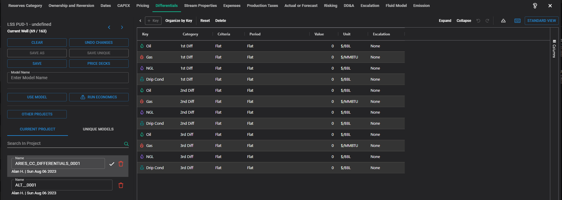 Advanced View

Differentials (Tab 6) 

- Supports Custom Streams

1st, 2nd and 3rd differential can be used to model increases or reductions in realized product pricing relative to basis (NYMEX).  These can be basin deducts, quality adjustments, use, access and marketing fees and other offsets.

1. Negative values indicate subtraction from price, positive a bonus to price.
   
2. You can copy/paste columns of data from Excel by clicking in a pricing cell and Ctrl-V.
   
3. Cap is value which the Escalation model will not let pricing exceed. 
   
4. Note that escalations occur on each entered time-series value and ONLY begin once the current value is in effect.  Values are not escalated from As of or the start of the escalation model but rather are only applied at the current escalation in effect during the period the values are being used.  
   
5. Note that the order of input on 1st, 2nd, 3rd differential governs calculation order rather than any notion of PEMDAS.  If both a dollar and a percent delta are both being used, the order of input can change the result.  For example, a $100 oil price with a -$5 1st and 90% 2nd differential will yield (100 - 5) * 0.9 = $85.50.  Flipping the order would be (100 * 0.9) - 5 = $85.00.
6. Begin Dates can be:
   
1. Flat: From As Of Date to ECL
   
2. As Of: From As Of Date and continuing for specified # months
   
3. Dates: From entered date.  Unless intended, be careful not to start after As Of Date
   

1. 1st Diff, 2nd Diff, 3rd Diff
   
1. Oil Differentials entered as:
   
1. $/BBL
   
2. % of Base Price Remaining
   
1. ie, 70% of $100 oil = $70 realized price
   
2. The % is applied to price continually as it changes per pricing model
   
2. Gas Differentials entered as:
   
1. $/MMBTU
   
1. Ensure BTU content defined in Stream Properties.
   
2. $/MCF
   
3. % of Base Price Remaining
   
1. ie, 70% of $5 gas = $3.50 realized price
   
2. The % applied to price continually as it changes per the pricing model
   
3. NGL Differentials can be entered as:
   
1. $/BBL
   
2. $/GAL
   
1. Since NGL Yield is set in Stream Properties at BBL/MMCF, 42 gal/BBL conversion factor applied in all calculations
   
3. % of Base Price Remaining
   
1. ie, 70% of $50 NGL price = $35 realized price
   
2. % applied to price continually as it changes per pricing model
   
3. Be careful not to double-dip if you have already applied reduction in oil price tab
   
4. Drip Cond Differentials entered as:
   
1. $/BBL
   
2. % of Base Price Remaining
   
1. ie, 70% of $50 Drip Cond = $35 realized price
   
2. The % is applied to price continually as it changes per pricing model
   
3. Be careful not to double-dip if already applied reduction in oil price tab
   

1. WTI-Brent Financial Futures
   
2. Argus LLS vs. WTI (Argus)
   
3. WTS (Argus) vs. WTI
   
4. WTI Midland (Argus) vs. WTI
   
5. WTI Houston (Argus) vs. WTI
6. WTS (Argus vws. WTI) ==> Deprecated, no longer traded or reported by CME
   
7. WRI Midland (Argus vs. WTI) ==> Deprecated, no longer traded or reported by CME
8. Clearbrook Bakken Sweet (NE2) ==> Deprecated, no longer traded or reported by CME
9. Edmonton Light Sweet (NE2) ==> Deprecated, no longer traded or reported by CME

 Standard View

 Advanced View

Stream Properties (Tab 7) 

- Supports Custom Streams

1. Date Triggers in all sections of this tab:
   
1. Flat: From As Of Date to Econ Limit
   
2. FPD : Begins at First Production Date
   
3. As Of : Begins at As Of Date applied in Dates section
   
4. Maj Seg : Begins when main phase starts prod
   
5. End Hist : Begins when well switches from actual historical data to forecasted data
   
6. Dates : Begins on scheduled date
   
7. Oil, Gas or Water Rate: Begins when prod crosses the threshold set for that one product.
   
1. Only “Gross Well Head” can be selected in this tab.
   
2. Monotonic or Non-Monotonic, is how variable production is treated with former not allowing rate changes on subsequent threshold crossings
   
1. Monotonic: Only decreases trigger changes. If forecast increases, no changes will be made to the value.
   
2. Non-Monotonic: The values look back up the schedule and vary with prod, up or down.
   

1. Yields
   
1. NGL Yield coincides with Gas Shrink since volume reduction occurs in the gas due to removal of the NGL.  The yield can be represented in one of two ways:
   
1. Unshrunk Gas (default): This is the measured BBL of NGL divided by the Produced Wellhead Gas.
   
2. Shrunk Gas: This is the measured BBL of NGL divided by the Gas sold .
   
2. Drip Condensate (retrograde condensate) is light oil produced from a gas well.  As a product ratio yield, no deductions through shrink or loss/flare taken. Drip Cond should not also be scheduled in the forecast section as “oil” and can be input here either as:
   
1. Unshrunk Gas (default): Volume condensate divided by wellhead gas
   
2. Shrunk Gas: Volume condensate divided by gas sold
   
3. Shrinkage
   
1. Oil Shrink is % volume fluid remaining caused by reduction in temperature and by the liberation of light ends as pressure is decreased.  Distinct from any oil losses occurring through other means.  This deduction affects only “Oil” and not “Drip Condensate”.
   
2. Gas Shrink coincides with NGL Yield since gas volume reduction is due to NGL removal. Usually calculated by sales gas divided by the wellhead gas produced (thus, % remaining, not % lost) at some aligned interval not including gas loss or flaring. If loss or flaring is transitory or measured separately, it should be reflected in the Loss/Flare Section.
   
4. Loss/Flare
   
1. Oil Loss - Volume % remaining after losses by anything other than normal shrinkage.  This reduction affects only “Oil” and not “Drip Condensate”.
   
5. Compositional Forecasting This tab is an interactive model which allows automatic calculation of shrinks and yields from known fractionation products.  However, it does not yet allow individual expenses to be applied against each product, only the resulting Gas and NGL.

In advanced view, this is moved into the normal window.  In standard, it is at the bottom of the screen.  Default is 1000 MBTU/MCF which means "do no adjustment"

1. BTU Content - Gas heating content relationship to produced volume.  Make sure correct if gas Pricing/Differentials are specified in $/MMBTU.
   
1. Unshrunk Gas (Wet Gas) impacts only variable expense (uncommon)
   
2. Shrunk Gas (Residue Gas) impacts revenues and possibly expenses depending on dropdown selections.

Standard View

Advanced View

Expenses (Tab 8) 

1. Criteria Triggers in all sections
   
1. Flat: From As Of Date to Econ Limit
   
2. FPD : Begins at the First Production Date
   
3. As Of : Begins at the As Of Date applied to the well in the Dates section
   
4. Disc Date: Begins at the Discount Date applied to the well in the Dates section
   
5. Maj Seg : Begins when main phase of the well starts production
   
6. End Hist : Begins when the well switches from actual historical data to forecasted data
   
7. Dates : Begins on a scheduled date
   
8. Oil, Gas Water Rate or Total Fluid: Begins when production crosses the threshold set for that one product.
   
1. Gross Well Head, Gross Sales, Net Sales volumes can trigger the changes
   
1. Monotonic or Non-Monotonic, is how variable production is treated with former not allowing rate changes on subsequent threshold crossings.  For instances when production forecasts have production that variably increases and decreases over time:
   
1. Monotonic: If production were to increase, no changes will be made to the value
   
2. Non-Monotonic: The values look back up the schedule and vary up or down depending on the production rate.
   

1. Variable Expenses - Variable expenses are normal operating costs based on a unit of production and often go away when a well is S/I such as treating, compression, etc.  They can be created in this section by:
   
1. Oil: $/BBL
   
2. Gas: $/MCF or $/MMBTU (If $/MMBTU, Ensure BTU content is defined properly in Stream Properties.)
   
3. NGL: $/BBL (not $/gal)
   
4. Drip Cond: $/BBL
   
2. Variable Expenses can be applied to five keywords for modeling:
   
1. G&P – Gathering and processing
   
2. OPC – Operating Costs (often used as a rollup of all other variable costs)
   
3. TRN – Transportation
   
4. MKT – Marketing
   
5. Other – Any cost bucket not defined above
   
6. Shrinkage Condition - Variable Expenses can be calc’d from volumes before or after shrink has been applied, so the corresponding condition should be selected to reflect which volume was used:
   
1. Unshrunk (default): Wellhead Production
   
2. Shrunk: Production sold
   
7. Calculation - Specify which interest to which the charges below apply.  Lease operating statements often dictate how they were initially calculated whether the statement was on a gross or WI basis.  Select:
   
1. 100% WI: (uncommon) Both the expenses and production are 8/8ths
   
2. LNRI: (common) The expenses are 8/8ths and the production denominator is based on the LNRI rather than the NRI for when it differs
   
3. WI: (default) The share of the expenses are to the WI and the production to the NRI
   
4. NRI: (uncommon) Both the expenses and production are to the NRI
   
5. Reversions: (uncommon) Any of the reversions listed on the Ownership and Reversions tab may be used according also to the explanations above.
   
1. Note: Projects imported from other platforms might default to NRI
   
8. Affect Econ Limit - Specify whether this expense is included in the well economic cutoff calculation (default is yes)
   
9. Deduct bef Sev Tax - If Severance Tax authorities allow a deduction for this expense, select yes. (default is No)
   
10. Deduct bef Ad Val Tax - If Ad Valorem Tax authorities allow a deduction for this expense, select yes. (default is No)
    
11. Cap - Cap is the maximum value not to be exceeded via the Escalation model.
    
12. Paying WI / Earning WI - Multiplier of WI for carried WI. Default is 1 for no carry. This generalized multiplier can be used in a variety of ways to adjust or risk Expenses by any fraction.
3. Fixed Expenses - Operating costs that stay persistent even when a well is S/I such as field salaries, trucks, etc.  They can be created in three buckets: Fixed 1,2, and 3 used interchangeably.
   
1. Unit
   
1. $/Month - Normal entry that does not get adjusted by well count (Assumed 1 for life)
   
2. $/Well/Month - New for v34 is the ability to enter a "well" schedule for multi-well leases and modeling purposes.  These are entered in the Risking Tab under Wells.  Selection here indicates the fixed cost is per-well which gets multiplied by the wells time-series array.
   
2. Adjustments
   
1. Affect Econ Limit - Specify whether this expense is included in the well economic cutoff calculation (default is yes)
   
2. Stop at Econ Limit - Should the fixed cost cease when economic limit is reached? (default is Yes)
   
3. Expense bef FPD - Should the fixed cost begin at the As Of date, or apply only after the well begins production? (default is No)
   
4. Deduct bef Sev Tax - If Severance Tax authorities allow a deduction for this expense, select yes. (default is No)
   
5. Deduct bef Ad Val Tax - If Ad Valorem Tax authorities allow a deduction for this expense, select yes. (default is No)
   
6. Cap - Cap is the maximum value not to be exceeded via the Escalation model.
   
7. Paying WI / Earning WI - Multiplier of WI for carried WI. Default is 1 for no carry. This generalized multiplier can be used in a variety of ways to adjust or risk Expenses by any fraction.
   
4. Water Disposal - A type of variable expense scheduled as $/BBL of water produced.  Therefore, water production must be set in the forecast section to apply costs here.
   
1. Note: Selections are similar to the above so echo those descriptions
   
2. Tip: You can use ELTs to enter a 2nd water disposal cost.  One input is allowed per input method: ie, one directly in the model, a second in an ELT, a third in yet another ELT.  Once "STANDARD VIEW" is deprecated, the prohibition on multiple key-category pairs will be removed.
   
5. Carbon (if you have Carbon Model Enabled) - Enter the expenses as $/MT

Production Taxes (Tab 9)

- Does NOT yet support custom Streams - so no prod tax available yet on those but coming soon.

1. Date Triggers in all sections
   
1. Flat: From As Of Date to Econ Limit
   
2. FPD : Begins at the First Production Date
   
3. As Of : Begins at the As Of Date applied to the well in the Dates section
   
4. Disc Date: Begins at the Discount Date applied to the well in the Dates section
   
5. Maj Seg : Begins when main phase of the well starts production
   
6. End Hist : Begins when the well switches from actual historical data to forecasted data
   
7. Dates : Begins on a scheduled date
   
8. Oil, Gas or Water Rate: Begins when production crosses the threshold set for that one product.
   
1. Gross Well Head, Gross Sales, Net Sales volumes can trigger the changes
   
1. Monotonic or Non-Monotonic, is how variable production is treated with former not allowing rate changes on subsequent threshold crossings.  For instances when production forecasts have production that variably increases and decreases over time:
   
1. Monotonic: If production were to increase, no changes will be made to the value
   
2. Non-Monotonic: The values look back up the schedule and vary up or down depending on the production rate.
   

1. State - A simplistic State Tax regime can be selected as a starting point.  These models have the default full-rate sev/adv taxes for each state but do not include:
   
1. tax holidays
   
2. interoperability of sev/adv deductions
   
3. reversions to lower taxes when the well reaches stripper status
   
4. The exception is when PA IF (Pennsylvania Impact Fee) for horizontal or vertical wells is selected, a PUC Schedule will show up with additional options. PA IF is imposed as $/year payment beginning the spud year of horizontal wells for the first 15-years.  Vertical wells are 20% of the horizontal fee for the first 10-years.  The schedule can be adjusted  annually by the PUC according to CPI and depends on the average gas price for the preceding calendar year. For modeling simplicity, monthly gas prices from the pricing inputs (no differentials) are used to determine the fee column.  If populated from the header or schedule, spud date is used to determine the years of service for the fee schedule but FPD can also be selected where appropriate.  For further reading, see: https://www.act13-reporting.puc.pa.gov/Modules/Disbursements/FeeSchedule.aspx 
1. Deduct Severance Tax, Shrinkage Condition and Calculation are irrelevant for PA IF.  By statute, the leaseholder pays the landowner's portion (WI).
2. Start Date (Note that a default hierarchy is followed: if you select "from headers" and it does not exist (null), CC will then use FPD as a backup.
   
1. SPUD Date from headers - The Spud Date from the headers for this well will be used.
   
2. SPUD Date from schedule - The Spud Date from the schedule module if that schedule is selected for this well in the Scenario.  WARNING!  CC schedules populate Spud ONLY when a spudder rig is used so it will be null otherwise.  A "Drill Start" will be added soon.
   
3. FPD - First production Date from the hierarchy in the "Dates" tab.
2. Severance Tax – Severance Taxes are state taxes on production.  Some apply the tax as a % of revenue, some as a price per unit of production , some both.  A price per month is also available.  Detailed schedules of severance tax holidays can be modeled as well as reversions to lower rates once the well reaches stripper status.
   
1. Calculation - Specify which interest to which the taxes below apply:
   
1. NRI: All parties receiving production pay their own share
   
2. WI: (uncommon) The lessor (landowner) share is paid by the lessee
   
3. Ad Valorem Tax - Ad Valorem Taxes are state or usually county/local tax assessed on the value of the production and/or equipment.  They can be modeled as a % of revenue, price per boe (at the conversion set for the project) or as price per month.
   
4. Deduct Severance Tax - Default is “No”.  Some taxing authorities allow Severance Tax deductions from Ad Valorem Tax calculation.
   
1. Calculation - Specify which interest to which the taxes below apply:
   
1. NRI: All parties receiving production pay their own share
   
2. WI: (uncommon) The lessor (landowner) share is paid by the lessee
   

Actual or Forecast (Tab 10)

- Has Advanced View (no Standard View)

- Supports Custom Streams

New for v36, this tab was converted to Advanced View with no button to select the old Standard View (migrated).  The old "Ignore Hist Prod" button has been deprecated in favor of moving it down into the selection of each item (thus allowing individual control of "never replace actuals with forecast".  

Note that selection of no model applied to wells will default to "Never" for all products.

Forecasts often overlap actual production records in a well.  Overriding actuals with forecast may be selected in each product with the trigger below

1. Key:
   
1. Select the product you wish to control: Oil, Gas Water or a Custom Stream that is previously created and appears in the dropdown.
   
2. Category:
   
1. Only available when a Custom Stream is selected to allow picking either: Company Custom Stream or Project Custom Stream
   
3. Replace Actual with Forecast Beginning On:
   
1. Never: Actual production is always used for economic calculations when there is overlap with a forecast (this includes "future production" in the case of volumetric forecasting.
   
2. Ignore Hist Prod - Since CC replaces actuals with forecasts, this button is intended to cover a circumstance for which there is no overlap of volumes: to ALWAYS ignore historical production if a forecasts exists over each month considered.
3. As Of Date: Forecast overwrite of actual production begins at the As Of Date selected in the Dates tab.
   
4. Date: Forecast overwrite of actual production begins on a scheduled date entered in the "Dates Value" header which only becomes available for entry when Date is selected.
   

Risking (Tab 11)

 - Does not yet support custom streams (except for "All" on Insert Shut-in Period covers Custom ALL streams including custom streams)

1. Risk Historical Prod - Default "Yes" - Applies the risking to any production entered in historical actual production (past or volumetric future volumes) that are after Aggregation Date.  Choose "No" to leave those unaffected.
2. Risk NGL & Drip Cond via Gas Risk - Default "Yes" - This selection adjusts the yield to risk before or after ratio products are calculated.  If "yes", Gas risk inherently risks NGL and Drip Condensate since they are input as a yield of Gas.  Selecting "No" will force explicit risking on those products independent of Gas. 
1. For example:
1. If Yes, gas 50% risk and NGL 50% risk means Gas 50% risk and NGL 25% risk. 
2. If No, Gas 50% risk and NGL 50% risk means Gas 50% risk and NGL 50% risk.
3. Risking - Risking is after Gross Wellhead Products schedules are calculated and are applied to Gross Sales Products.  
1. For instance: 100 Mcf/d risked 50%:
1. Gross WH = 100 Mcf/d
2. Gross Sales = 50 Mcf/d
3. Products:
1. Oil
2. Gas
3. NGL
4. Drip Cond
4. Methods
1. Flat: From As Of Date to Econ Limit
2. FPD: Begins at the First Production Date
3. As Of: Begins at the As Of Date applied to the well in the Dates section
4. Maj Seg: Begins when main phase of the well starts production
5. End Hist: Begins when the well switches from actual historical data to forecasted data
6. Dates: Begins on a scheduled date
7. Seasonal : This opens up a Month-of-Year schedule with defaults of 100%.  Adjustments can be made for seasonality for things like winter freeze-offs, elk-migration, etc.  Care should be taken to average 100% year-round unless modeling additional reduction/enhancement rather than just shifting of EUR is desired.
4. Wells: This is not technically a "Risking" but rather an adjustment of the number of wells represented by the modeled property.  This can be used for accumulated leases whereby the production historical and forecast represents many wells.
1. Purpose: Wells has three functions: 
1. When "$/Well/Month" is used as the Fixed Cost in the Expense Tab, the fixed cost is multiplied by this wells time-series array.
2. Econ Run well counts are integrated to account for the number of wells on a lease.  These may be viewed on any aggregated report
3. Econ Group - when "Well Count" is selected as the Allocation Method Type on the input screen, the number of wells adjusted here will appropriately be weighted when considering how to allocate the group input to the individual properties.
2. Input
1. Count: Absolute number or time-series each period of wells 
2. Percentage: The first number entered is the beginning count and then the remaining are time-series adjustments by multiplying a percentage against the original count.
3. Methods: Same as risking except for no "Seasonal"
4. Note, the entry is robust for specific modeling and allows:
1. Decimal number of wells for fine-tune adjustment or averaging
2. (0) Zero wells may be used to nullify fixed expenses and avoid incrementing output well counts
3. Negative wells may be entered to flip the sign of fixed expenses and de-increment well counts
5. Insert Shut-in Period - Scenario method to SI a well temporarily for adjustment.  This is in addition to any SI Period used in the forecasting module.
1. Shut-in periods can be scheduled for one or all product phases in a well to account for known upcoming or averaged unknown events.  Scheduling a shut-in will cause production to cease for a period and return to the next scheduled production rate after that period expires.
1. As Of: Starting # days from the As Of date to # days from the As Of date. (ie, As Of plus 100 days to 200 days)
2. Dates: Begin date of shut-in to end date of shut-in.
2. Scale Post Shut-in can be used to return the well at a reduced or enhanced production rate and percentage of remaining reserves from that point. (ie, for a well making 1 MMcf/d with remaining reserves of 1 bcf, a scale factor of 0.5 applied would return the well at 0.5 MMcf/d and 0.5 Bcf reserves.  However, economic cutoff might then further reduce reserves.)
1. Scale Post Shut-In End Criteria - The point at which to stop reflecting that scalar and return to the default: 1
2. Fixed Expenses and CAPEX defaults are “Yes” and allow scheduled charges to occur during the shut-in period.  Per unit production charges such as variable expenses and production tax (%) will not be applied during the shut-in period.
3. Note: Shut-in Period can be used to model curtailment.  If you enter one day SI per month and repeat, this works similarly to preserve EUR by truncating the forecast at that point and picking up at the next scheduled production point at the end of the SI period.  So this would be a quanta of 1/30.4375 (3.29% Curtailment) for each repeated day per month (on average as it would change by the number of days in each month).  Increase the number of days each month to scale the curtailment.  Note that using this method will sometimes slow economic calculation speed.  Full curtailment support is planned for a future release.
4. Note: Interaction with any cutoff method selected in the dates tab may affect total remaining reserves.
5. Note: Care should be taken not to cross months/years using the repeater in such a way as to create an illogical or inconsistent condition.  Some validation exists to avoid this.  For example: having a SI from 1/1 to 3/1 and repeating monthly is illogical as is a SI from 2/20 to 3/4 and repeating monthly.

DD&A (Depreciation, Depletion & Amortization) (Tab 12) 

- Note: tab is not listed in the Scenario Page for selection but only within the "Econ Editing" tabs.

Note: to enable output of AFIT (After Federal (and State) Income Tax calculations in CC, you must select "Income Tax" = "yes" in General Options for that model applied to the current scenario.  General Options is also where you can apply a 15% Percentage Depletion in lieu of Cost Depletion, (NOL) Carry Forward (yes/no), State and Federal Income Tax multipliers as time-series.  See the discussion on the General Options section for these items.

Depreciation Models apply tax recovery schemes over time in economic variables and are named/numbered as Project or Unique for reference by selection in the Investment (CAPEX) tab.  Tangible and Intangible amounts are entered and tax-treated independently via that applied model.  Only one Model Type may be selected at a time for application on an Investment line in CAPEX so it is recommended to name the models with the type selected like "Depletion: UOP-mp", etc.  The type of investment selected will dictate the Model type applied. 

1. Model Type: Choose to create a model for CAPEX items to either be Depreciated, Depleted or expensed.
1. Expensed items such as same-zone workovers which are written off in the first year, can have no DD&A model applied or just a depreciation model with 100% in year 1
2. Depreciated items such as Drilling can have separate schedules applied on the tangible or intangible portions as defined in the CAPEX model.  Several built-in schedules can be populated and edited.
3. Depleted items such as initial purchase price can be deducted against income for taxation by several methods
   

1. Depreciation Model Type
   
1. Pre-built Depreciation Model - Note MACRS stands for the preferred amortization method used for scheduled depreciation: "Modified, Accelerated Cost Recovery System".  
   
1. MACRS 3, 5, 7, 10, 15, 20 Year schedules are available for pre-filled percentages in one extra increment (ie, 7-year = 8 periods) due to the "half-year convention" which starts the schedule on July 1 of the first year of deduction.  MACRS 7 Year is most common in oil and gas applications.
   
2. Custom allows entry of your own schedule with any number of rows.  Ensure the total Cumulative percentages for Tan and Intan always add up to 100%
   
2. % Tangible Fed Tax Credit - Immediate tax credit (CAPEX times credit %).  This is independent of any other deduction (applied "on the top")
   
3. Bonus Depreciation - In addition to any schedule percentages below, take a percentage of the total as a time-0 deduction.  Note: The remaining scheduled factors should still add up to 100% as they are percentages of the remaining AFTER Bonus Depreciation methods.
1. TCJA Bonus Depreciation - Default "No" will allow only manual Bonus Depr entry.  "Yes" applies Bonus Depr from this Tax Cuts and Jobs Act schedule by investment year:
   
1. 2010-11: 100%
   
2. 2012-17: 50%
   
3. 2018-22: 100%
   
4. 2023: 80%
   
5. 2024: 60%
   
6. 2025: 40%
   
7. 2026: 20%
   
8. 2027+: 0%. 
   
9. Don't double-dip with manual Bonus entry.  TCJA is intended to be stand-alone, not double-dipped with manual Bonus Depr entry.  The Pre-built Depr Models are the % factors applied on the remaining amount after all bonus.
   
2. % Tangible Bonus Depreciation and % Intangible Bonus Depreciation - If TCJA is not used, allows manual selection of an immediate deduction.
   
4. Depreciation - The Tangible and Intangible schedules reflected here from the Pre-built Depreciation Model above.
   
2. Depletion Model Type - Depleted items such as initial purchase price can be deducted against income for taxation by several methods and applied separately for the amounts located in tangible (for modeling purposes only since tangible items are never depleted) and intangible.  Be mindful when 15% Percentage Depletion is selected in General Options as the greater of that or the applied method below will be used in CC calculations.
   
1. % Tangible or % Intangible Immediate Deduction - Amount of CAPEX to take as a depletion deduction at spend date.  Any remaining amount will be deducted via the method below.
   
2. Tangible Cost or Intangible Cost Depletion Model
   
1. UOP (Major Phase) - Units of Production which is the current monthly production of the major phase divided by EUR times the running balance of the basis.
   
2. UOP (BOE) - Units of Production which is the current monthly production of the well using the BOE factor divided by EUR times the running balance of the basis.
   
3. Deduct at Economic Limit - For items that can't be written off until plugging, sale, etc.
   
4. No Depletion - Do not deduct any depletion for this particular item.
   
5. Expense at FPD - Deduct 100% of the entire amount in the year the expenditure is made.
   
3. Note: Tangible, Depletable does not exist in reality as an asset class. However, it can be used as a separate bucket to deduct differently via a tan/intan split model to tax-treat each via separate method.

Note: Run Scenario - Economics Runs auto-select some AFIT items when AFIT "Income Tax" = "yes" is selected in General Options but many more (45) items may be output on the "Columns" selection of the Run Scenario screen.

Escalation (Tab 13) 

- Note: tab is not listed in the Scenario Page for selection but only within the "Econ Editing" tabs.

1. Escalation Models allow defined increase or decrease over time in economic variables and are named/numbered as Project or Unique for reference by selection in the other tabs such as:
   
1. CAPEX & other Investments
   
2. Pricing and Differentials
   
3. Expenses and Production Taxes
   
2. Note that “Caps” can be set to override escalation via maximums in the Pricing and Expenses tabs.
   
3. Escalation is either be set to increment by % per year or $ per year ($ Escalations are always simple by period though).  The Escalation Frequency can change either Monthly or Yearly increments.  The Compound Method can be either Compound or Simple(Linear). Example: assuming a % escalation, the four following  models could be created at +10% APY of a $1000 per month expense for 3-years:
   
1. Monthly Simple: $100 is added every year but is applied monthly as $100/12=$8.33 added each month
   
2. Monthly Compound: Each month increases by multiplying the previous by 10%/12 and adding the previous month total.
   
3. Yearly Simple:  Every 12th month increases $100 (12-mo @ $1000, 12 @ $1100, 12 @ $1200)
   
4. Yearly Compound: Every 12th month increases 10% over preceding month (like 12-mo @ $1000, 12 @ $1100, 12 @ $1210)
   
4. New for v36 - Calculation Method was added to give greater control over time-series lines in all tabs.  A dropdown with the following:
   
1. Also, be aware that any selection made here of "Adjust All From Date" will override the same type of start control given explicitly in the CAPEX model Escalation Start.  Selection of "Adjust Active Series" will leave full control on the CAPEX Escalation Start Option in the CAPEX tab.
   
2. Adjust Active Series (default and historically, the only method) - this only escalates a time-series line (like $2000 fixed expense for 1-year, then $3000 thereafter) while it is being actively used (in service for the rolling calculated month being investigated in econ.  Therefore, the $3000 fixed expense would come in at $3000 even if your escalation scheme started many years before that date.  This method would be good for a model of "I know what I want until the end, then escalate the last value thereafter".
   
3. Adjust All from Date - new feature to start ALL escalation lines from a specified date.  So each time-series would be pre-escalated if the date here as well as the scheme started before the line came into service.
   
1. FPD - Same as Date below but auto-adjust the start date to be equal to the FPD returned from the hierarchy in the dates tab.
2. As of - Same as Date below but auto-adjust the start date to be equal to the As of selection in the dates tab.
   
3. Date - Allows entry of a date on a pop-in row of "Adjust Start Date".  This method would be good for a model of "I know what my expenses are today but if a well starts in many years, I want those escalated to account for inflation".
5. Flat, Month Period (# months from As Of), or Dates (From-To) may be selected to define the period of escalation.  
   
1. Use of the "Adjust..." date set to FPD and "Month Period" here might be a good way to model "I want the expenses to stay the same but start escalating when the well starts".
6. More complex models are possible to schedule via the plus icon but one scheme (monthly/yearly & simple/compound & %/$) is allowed per model
   
7. Note that positive escalation increases (inflates) numbers over time and negative escalation decreases (deflates) numbers over time.   Whether this increases or decreases depends on where it is applied: positive escalation increases NPV for pricing but decreases NPV for expenses for example.
   
8. Tip: The Escalation Frequency, “constant” is a legacy keyword and should not be used.
   
9. Tip: The Combo Curve importer does a good job pulling in escalation schemes from Access databases originating in other economics packages.  Ideally, continuation lines are the preferred method of scheduling complex schemes for efficient import.  Note that some escalation schemes are not yet supported in CC such as Expense escalation of all time-series lines from time-0; escalation is only applied on each time-series line as it is in "use" so this differs from other economics packages.  Independently applying disparate escalation schemes to individual time-series lines is also not yet supported.
   
10. Note no escalation is exported to other software packages.  It is imported from those packages however.
    

Fluid Model (Tab 14) 

1. Please refer to the Fluid Model section of the Carbon Network Overview article.
   

Emission (Tab 15) 

Emission models allow you to assign top-down (high level) emission estimates to wells in a scenario. These emissions include all emission categories in EPA Subpart W, categories not specifically covered in EPA Subpart W (Scope 2 and Scope 3), and categories that are reported within other EPA categories (Drilling Combustion and Completion Combustion).

Top-down emissions are defined as either a carbon dioxide equivalent (CO2e) or in any combination of carbon dioxide (CO2), methane (CH4), and nitrous oxide (N2O). CO2e cannot be used in combination of the other 3 gases since CO2e is calculated directly from those 3 gases when they are available. Refer to the Global Warming Potentials section of the Carbon Network Overview article for the calculation methodology.  For each desired category, define the mass of greenhouse gas emissions in the unit of metric tons (MT) per unit of activity relevant to that emission category. These units are:

1. MT/MBBL: For emissions related to oil production volume, such as atmospheric tanks.
2. MT/MMCF: For emissions related to gas production volume, such as flare.
3. MT/MBOE: For emissions related to oil equivalent volume.
4. MT/Well/Year: For recurring emissions that apply to each well, for example the lighting of the well pad that is required regardless of activities or production volumes. Emissions allocated on a monthly basis based on the number of days in each month.
   
5. MT/New Well: For emissions that occur once, when the well is put online (at or near FPD), such as drilling and completion. Emissions will be calculated at FPD, as defined in the Dates model.
   

Use the Escalation field to model desired changes to emissions with time. For example, to model replacing 50% of pneumatic pumps in March 2024 with non-emitting pumps, define an escalation model in the Escalation tab with 50% reduction (-50%) occurring in 03/2024 and assign it to the Pneumatic Pump category.

Tip: Add an additional row of the same category using the +Row button. An additional row is added to the bottom of the table. Change the category by double-clicking on the category name and selecting another category from the dropdown. Having multiple rows for the same category is useful when an emission depends on multiple factors, for example electricity (Scope 2) could be used for both gas compression and for lighting.  Enter the electricity for gas compression with MT/MMCF and the electricity for lighting with MT/Well/Year.

Import Emissions

ComboCurve provides an automated way to input values into an Emission model based on prior year submitted EPA reports. We have scraped (downloaded) all publicly available Subpart W EPA reports back to 2015 for all oil and gas companies in all basins and have normalized those emissions by well count and production volumes . You can use values from your own EPA reports from prior years or model neighboring operators for comparison and benchmarking. Press “Import Emissions” and a dialog opens to choose the desired reporting year, company, basin, and emission categories to import.

 

Once applied, the table is populated with appropriate emission values for the applicable greenhouse gases in units predetermined to match the nature of each emission category. Toggle each emission category on and off to use or ignore that category in the Carbon run.

Emission models can be used alone or in combination with Carbon Network models. Emissions for each well and month are aggregated from the Carbon Network and Emission model assigned in the Scenario table. To avoid double counting emissions for a well from the same categories in both a Carbon Network and an Emission model, toggle off the categories from the Emission model.

Example: Import emissions from a previous year’s EPA report as a baseline. Toggle off the Associated Gas, Pneumatic Device, Atmospheric Tank, and Reciprocating Compressor categories in the Emission model and then define those categories using nodes in a Carbon Network with detailed Fluid Models, equipment counts and runtimes.